ECON 4370 / 6370 Computing for Economics

Lecture 7: Spatial Data and GIS

Zhan Gao

14 September 2026

Location changes the question

Familiar data question	Spatial version
Which county has more births?	Where are births concentrated?
Which observations belong together?	Which departments does a river cross?
How do outcomes vary across units?	Do nearby villages share similar outcomes?

A map adds location. A spatial operation makes location part of the analysis.

Today’s route

1. Features and coordinates: read a map and understand its CRS.
2. Wrangling and measurement: reuse tidyverse tools and measure geometry.
3. Spatial relationships: distinguish filtering, joining and intersecting.
4. Research examples: map villages and join county attributes.

Projection and data-access examples follow the main lesson.

The lecture focuses on vector data. Raster analysis and spatial econometric estimation are beyond this session. Build on the unit-of-observation discussion in lecture 6.

Packages and data

Run the examples from the lectures/ directory.

library(sf)
library(tidyverse)

Example	Source
North Carolina counties	Shapefile bundled with sf
French departments and rivers	maps and spData
World and country outlines	rnaturalearthdata
Village outcomes	data/china_map_dt.Rdata
County treatment fields	data/counties_treated.Rdata

Use maps::map() explicitly: purrr also has a function called map().

Features and coordinates

---

A data frame with a geometry column

What is a spatial feature?

A feature combines attributes, geometry, and a coordinate reference system (CRS).

Geometry	Example	Attributes
Point	A village	ID, migration share
Line	A river	Name, length
Polygon / multipolygon	A county, possibly with islands	FIPS code, birth count

In an sf data frame, one row describes one feature. Its coordinates live in a geometry list-column.

[Sources] - https://r-spatial.github.io/sf/articles/sf1.html A multipolygon can contain several disconnected polygon pieces in one feature. Vector data represent discrete features; a raster stores values on a grid.

Read a shapefile

file_loc <- system.file("shape/nc.shp", package = "sf")
nc <- st_read(file_loc, quiet = TRUE)

nrow(nc)

## [1] 100

st_geometry_type(nc) %>% as.character() %>% table()

## .
## MULTIPOLYGON 
##          100

st_read() also reads formats such as GeoPackage and GeoJSON.

A shapefile is a set of files. Keep its .shp, .shx, .dbf, and available .prj files together.

[Sources] - https://r-spatial.github.io/sf/articles/sf2.html The package supplies all components in the same folder. For a new project, record the provider, geography vintage and CRS.

Inspect attributes and spatial metadata

nc %>% select(NAME, FIPS, BIR74) %>% slice_head(n = 3)

## Simple feature collection with 3 features and 3 fields
## Geometry type: MULTIPOLYGON
## Dimension:     XY
## Bounding box:  xmin: -81.74107 ymin: 36.23388 xmax: -80.43531 ymax: 36.58965
## Geodetic CRS:  NAD27
##        NAME  FIPS BIR74                       geometry
## 1      Ashe 37009  1091 MULTIPOLYGON (((-81.47276 3...
## 2 Alleghany 37005   487 MULTIPOLYGON (((-81.23989 3...
## 3     Surry 37171  3188 MULTIPOLYGON (((-80.45634 3...

• 100 rows: one per North Carolina county.
• MULTIPOLYGON: each feature can contain several polygon pieces.
• NAD27 / EPSG:4267: longitude and latitude in degrees.
• geometry: the coordinates needed to draw each county.

Geometry stays with the data

county_names <- nc %>% select(NAME)
names(county_names)

## [1] "NAME"     "geometry"

nc %>%
  st_drop_geometry() %>%
  select(NAME, FIPS) %>%
  slice_head(n = 3)

##        NAME  FIPS
## 1      Ashe 37009
## 2 Alleghany 37005
## 3     Surry 37171

select() keeps the geometry attached. Use st_drop_geometry() when you want an ordinary table.

[Sources] - https://r-spatial.github.io/sf/reference/tidyverse.html

Draw the first map with geom_sf()

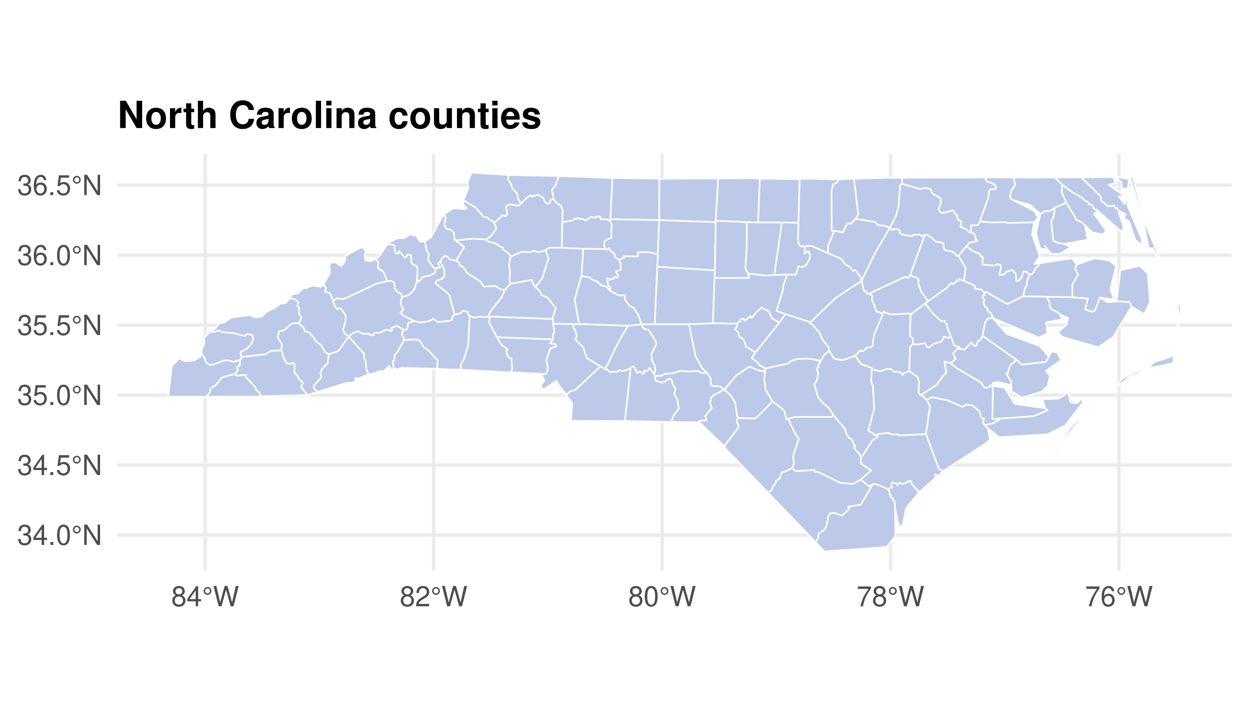
nc_outline <- ggplot(nc) +
  geom_sf(fill = "#BDC9E8", colour = "white", linewidth = 0.3) +
  labs(title = "North Carolina counties") +
  theme(axis.title = element_blank())
nc_outline

geom_sf() reads the geometry column; no x or y mapping is needed.

One feature per county

The map places the same rows we inspected in geographic space.

Coordinates, wrangling and measurement

---

Coordinates need a reference system and units

A CRS gives coordinates meaning

A CRS specifies how coordinate values relate to Earth, including the reference datum, axes and units.

CRS type	Coordinates	Example
Geographic	Longitude / latitude, usually degrees	NAD27, EPSG:4267
Projected	Planar coordinates, often metres	NAD83 / North Carolina, EPSG:32119

Every flat map distorts some combination of area, shape, distance or direction.

Choose a CRS for the study region and task. A visually familiar map is not automatically suitable for measurement.

[Sources] - https://r-spatial.github.io/sf/reference/st_crs.html - https://proj.org/en/stable/usage/projections.html EPSG identifiers and WKT are convenient complete CRS specifications. A projection name alone does not identify all CRS parameters.

Transform the coordinates

st_crs(nc)$input

## [1] "NAD27"

nc_m <- st_transform(nc, 32119)
st_crs(nc_m)$units_gdal

## [1] "metre"

st_bbox(nc_m) %>% round()

##   xmin   ymin   xmax   ymax 
## 123830  14740 930519 318256

nc_m now uses a projected North Carolina CRS with coordinates in metres.

The county attributes and feature count stay the same.

Assigning a CRS is a different operation

Function	What changes?	When to use it
st_crs(x)	Nothing; inspects metadata	Check the existing CRS
st_set_crs(x, ...)	CRS metadata only	Attach the known source CRS
st_transform(x, ...)	Coordinate values and CRS	Convert from a known CRS to another
coord_sf(crs = ...)	Plot display	Draw a map in another CRS

Relabeling degree coordinates as metres does not reproject them.

[Sources] - https://r-spatial.github.io/sf/reference/st_crs.html - https://ggplot2.tidyverse.org/reference/ggsf.html

Compute area with explicit units

nc_m <- nc_m %>%
  mutate(area_km2 = as.numeric(
    units::set_units(st_area(geometry), km^2)
  ))

nc_m %>%
  st_drop_geometry() %>%
  select(County = NAME, `Area (km²)` = area_km2) %>%
  slice_head(n = 3) %>%
  knitr::kable(digits = 1)

County	Area (km²)
Ashe	1137.6
Alleghany	611.2
Surry	1423.7

The bundled AREA column is a legacy field. Compute physical area from geometry and keep track of its units.

[Sources] - https://r-spatial.github.io/sf/reference/geos_measures.html - https://search.r-project.org/CRAN/refmans/spData/html/nc.sids.html The original AREA field is in degree units. These are projected polygon areas, not a measurement of land area excluding inland water. The chosen state-plane projection has small local distortion, not exact global area preservation.

Familiar dplyr verbs still work

selected <- nc_m %>%
  filter(NAME %in% c("Camden", "Durham", "Northampton")) %>%
  mutate(births_per_km2 = BIR74 / area_km2) %>%
  select(NAME, area_km2, births_per_km2)

selected %>% st_drop_geometry() %>%
  knitr::kable(digits = 1,
    col.names = c("County", "Area (km²)", "Births per km²"))

County	Area (km²)	Births per km²
Northampton	1521.0	0.9
Camden	616.0	0.5
Durham	770.5	10.3

This is a spatial concentration measure for the recorded period, not a birth rate per person.

Check the codebook before comparing years

The NC data contain birth totals for two periods:

Field	Coverage	Duration
BIR74	July 1974–June 1978	4 years
BIR79	July 1979–June 1984	5 years

A larger total in BIR79 could partly reflect the longer observation window. These are not single-year counts.

The same caution applies to differences in county population size.

[Sources] - https://r-spatial.github.io/spdep/articles/sids.html This is a historical teaching dataset. The lecture uses births to demonstrate reshaping and mapping, not to infer changes in fertility.

Reshape attributes; keep the polygons

nc_births <- nc_m %>%
  select(NAME, BIR74, BIR79) %>%
  pivot_longer(c(BIR74, BIR79),
               names_to = "period", values_to = "births") %>%
  mutate(period = recode(period,
    BIR74 = "1974–78 (4 years)",
    BIR79 = "1979–84 (5 years)"))

nrow(nc_births)

## [1] 200

There are now 200 rows: one county–period per row, with the county geometry repeated for each period.

Facet maps with the same grammar

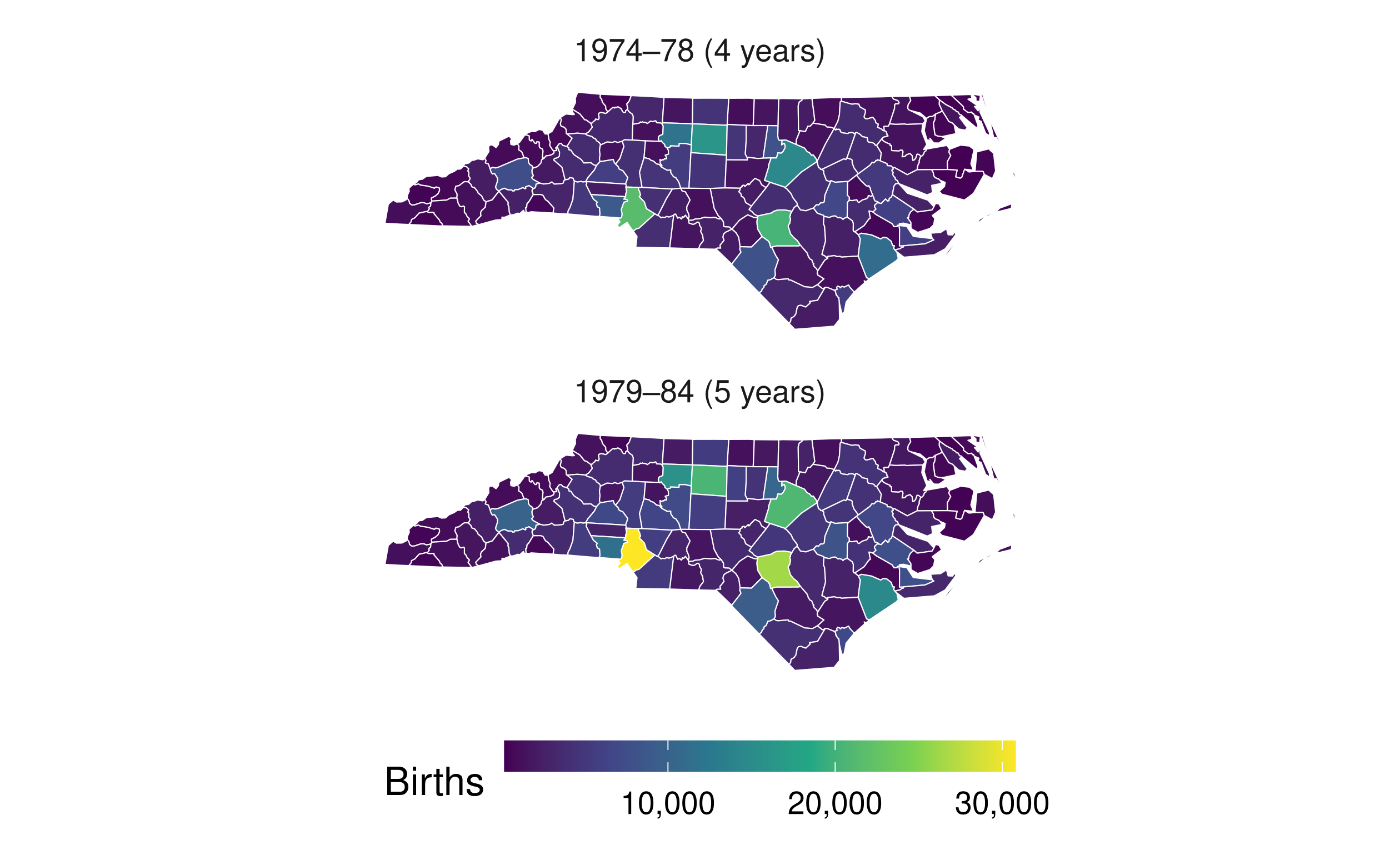
ggplot(nc_births) +
  geom_sf(aes(fill = births), colour = "white") +
  scale_fill_viridis_c(name = "Births", labels = scales::comma) +
  facet_wrap(~period, ncol = 1) +
  coord_sf(datum = NA)

Geometry supplies the map. fill and facet_wrap() use the reshaped attributes, with one shared colour scale.

Map the same measure across periods

Visible plotting recipe: ggplot(nc_births) + geom_sf(aes(fill=births)) + facet_wrap(~period). A common scale allows comparison of recorded totals; the unequal periods and county populations still matter for interpretation.

Check your understanding

1. What does one row represent before and after pivot_longer()?
2. Why does select(NAME) still let you draw a map?
3. Why would st_set_crs(nc, 32119) be wrong here?
4. What additional information would you need to compare birth rates across counties?

Answers: county versus county–period; sticky geometry; assignment would mislabel unchanged degree coordinates; a relevant population denominator and a consistent time period.

Operations on geometry

---

Measure or construct features

What can we do with one layer?

Function	Output	Example use
st_area()	Measurement with units	County area
st_centroid()	Point geometry	Geometric centre
st_point_on_surface()	Point on the feature	Place a polygon label
st_buffer()	Expanded geometry	A distance-based zone
st_union()	Combined geometry	Dissolve county boundaries

For planar operations, use a suitable projected CRS and check its units.

[Sources] - https://r-spatial.github.io/sf/reference/geos_unary.html A polygon centroid can fall outside a concave or multipart polygon. A buffer is geometric proximity, not travel distance or a causal treatment definition.

Compute centres in projected coordinates

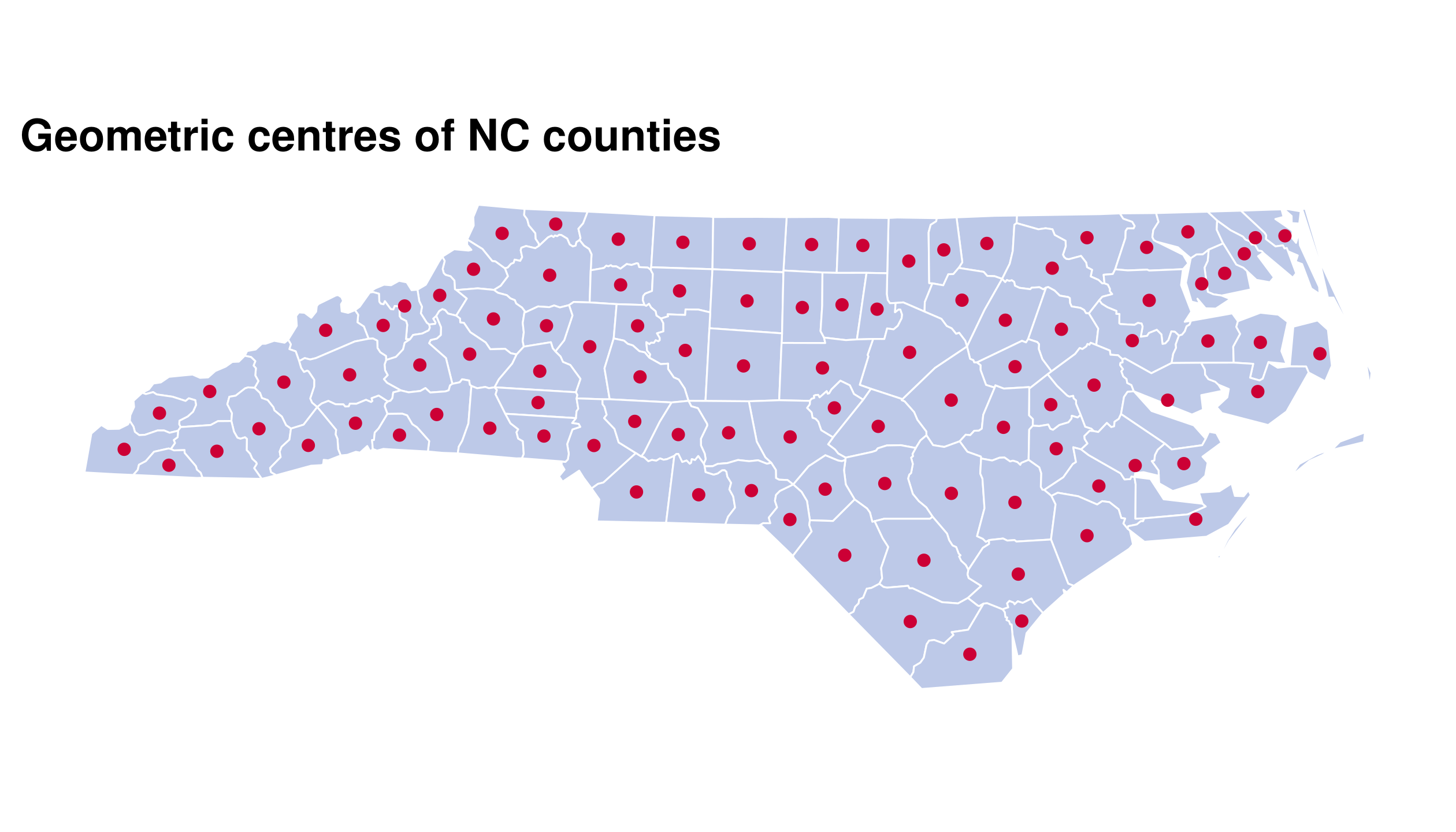
centres <- st_centroid(st_geometry(nc_m))

centres_map <- ggplot(nc_m) +
  geom_sf(fill = "#BDC9E8", colour = "white", linewidth = 0.3) +
  geom_sf(data = centres, colour = "#CC0035", size = 1.5) +
  coord_sf(datum = NA) +
  labs(title = "Geometric centres of NC counties")
centres_map

These are geometric centres, not county seats or population centres.

Centroids summarize polygon geometry

A centroid can lie outside a polygon. For a label that must lie on the feature, use st_point_on_surface().

Dissolve internal boundaries

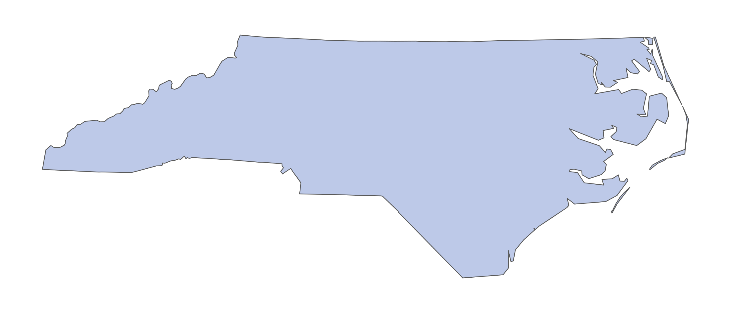
nc_border <- st_union(nc_m)
ggplot() + geom_sf(data = nc_border, fill = "#BDC9E8") +
  coord_sf(datum = NA)

st_union() combines geometry. It does not automatically produce meaningful totals for the original county attributes.

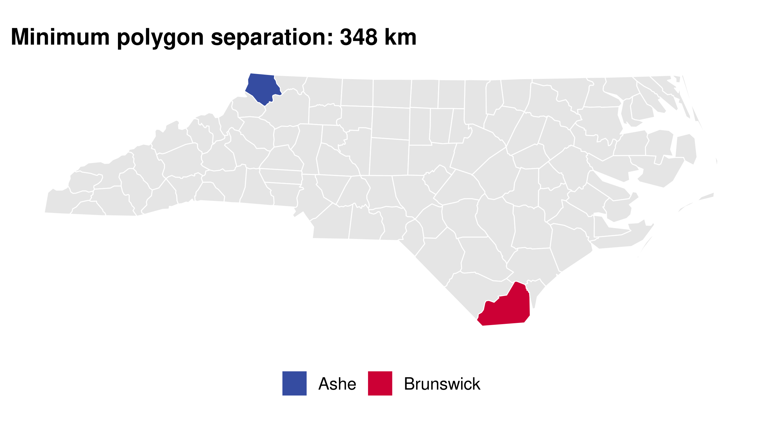
Specify what distance means

ashe <- nc_m %>% filter(NAME == "Ashe")
brunswick <- nc_m %>% filter(NAME == "Brunswick")

distance_km <- st_distance(ashe, brunswick) %>%
  units::set_units(km)
round(distance_km, 1)

## Units: [km]
##       [,1]
## [1,] 347.9

This is the minimum separation of the two county geometries in the projected CRS.

It is not a driving distance or the distance between county seats. Adjacent polygons have distance zero.

[Sources] - https://r-spatial.github.io/sf/reference/geos_measures.html st_distance returns a pairwise matrix by default. by_element=TRUE requires paired objects of equal length. Spherical or ellipsoidal distances can differ slightly from this projected result.

The objects define the distance

Spatial relationships

---

Which departments does a river cross?

Align the layers before combining them

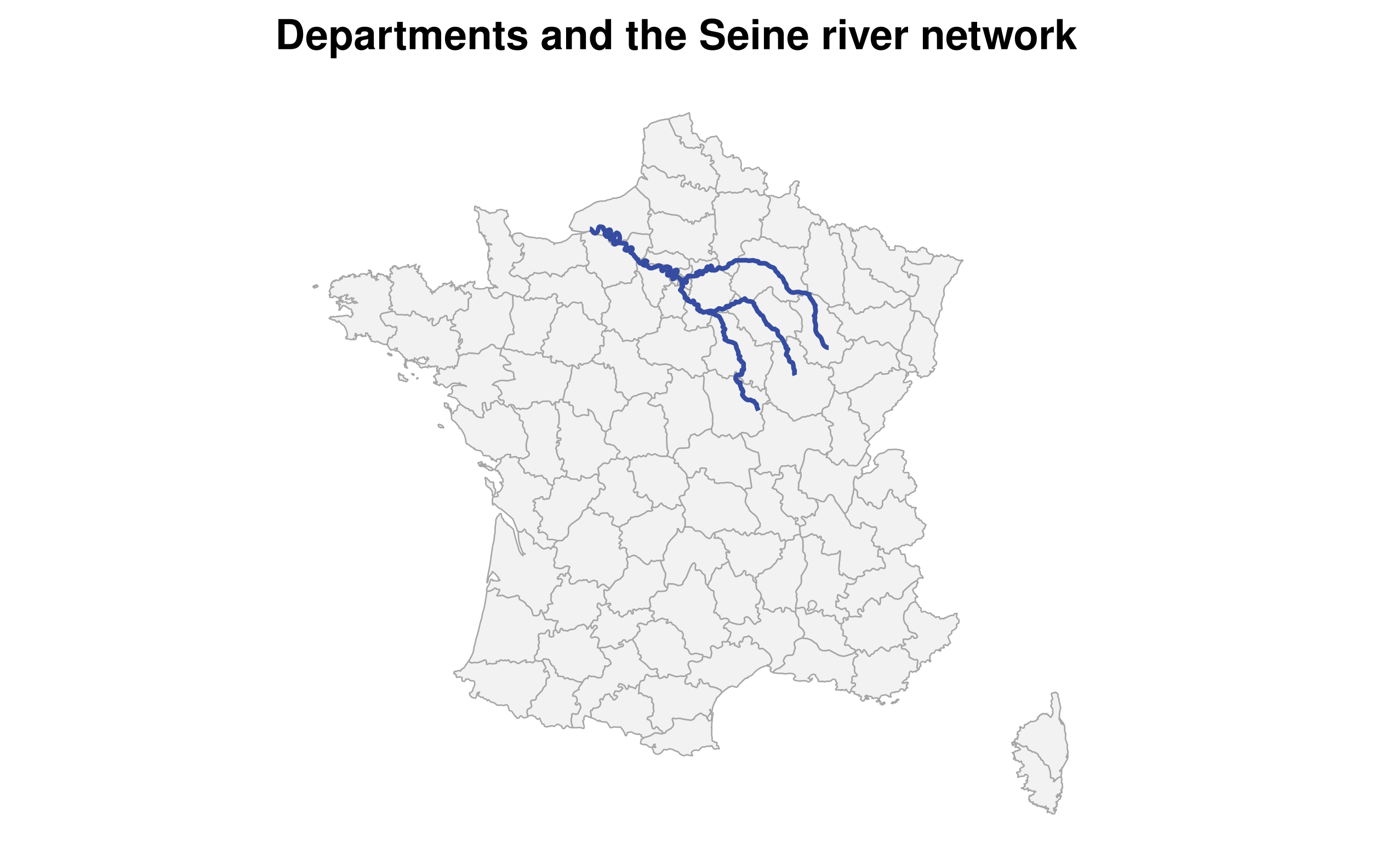
france <- maps::map("france", plot = FALSE, fill = TRUE) %>%
  st_as_sf() %>% st_transform(2154) %>% st_make_valid()
seine <- spData::seine %>%
  st_transform(2154) %>% st_make_valid()

st_crs(france) == st_crs(seine)

## [1] TRUE

all(st_is_valid(france))

## [1] TRUE

Both layers now use RGF93 / Lambert-93, a projected CRS for metropolitan France.

The maps layer contains historical departments, not current administrative regions.

[Sources] - https://search.r-project.org/CRAN/refmans/maps/html/france.html - https://r-spatial.github.io/sf/articles/sf7.html The maps France source is historical NUTS III boundaries, circa 1989, supplied by UNESCO through UNEP/GRID-Geneva. spData supplies the Seine, Marne and Yonne lines. Projected operations use GEOS; no global S2 toggle is needed.

Two layers, two kinds of features

A predicate tests a spatial relationship

hits <- st_intersects(france, seine)
france_hits <- france %>% mutate(n_rivers = lengths(hits))

france_hits %>% st_drop_geometry() %>%
  count(n_rivers, name = "Departments") %>%
  knitr::kable(col.names = c("Intersecting river features", "Departments"))

Intersecting river features	Departments
0	79
1	13
2	3
3	1

st_intersects() returns matches, not a new map geometry. A department may intersect more than one river feature.

[Sources] - https://r-spatial.github.io/sf/reference/geos_binary_pred.html The default result is a sparse list: element i contains the matching row numbers from the second layer. Boundary contact counts as intersection.

Filter to whole matching departments

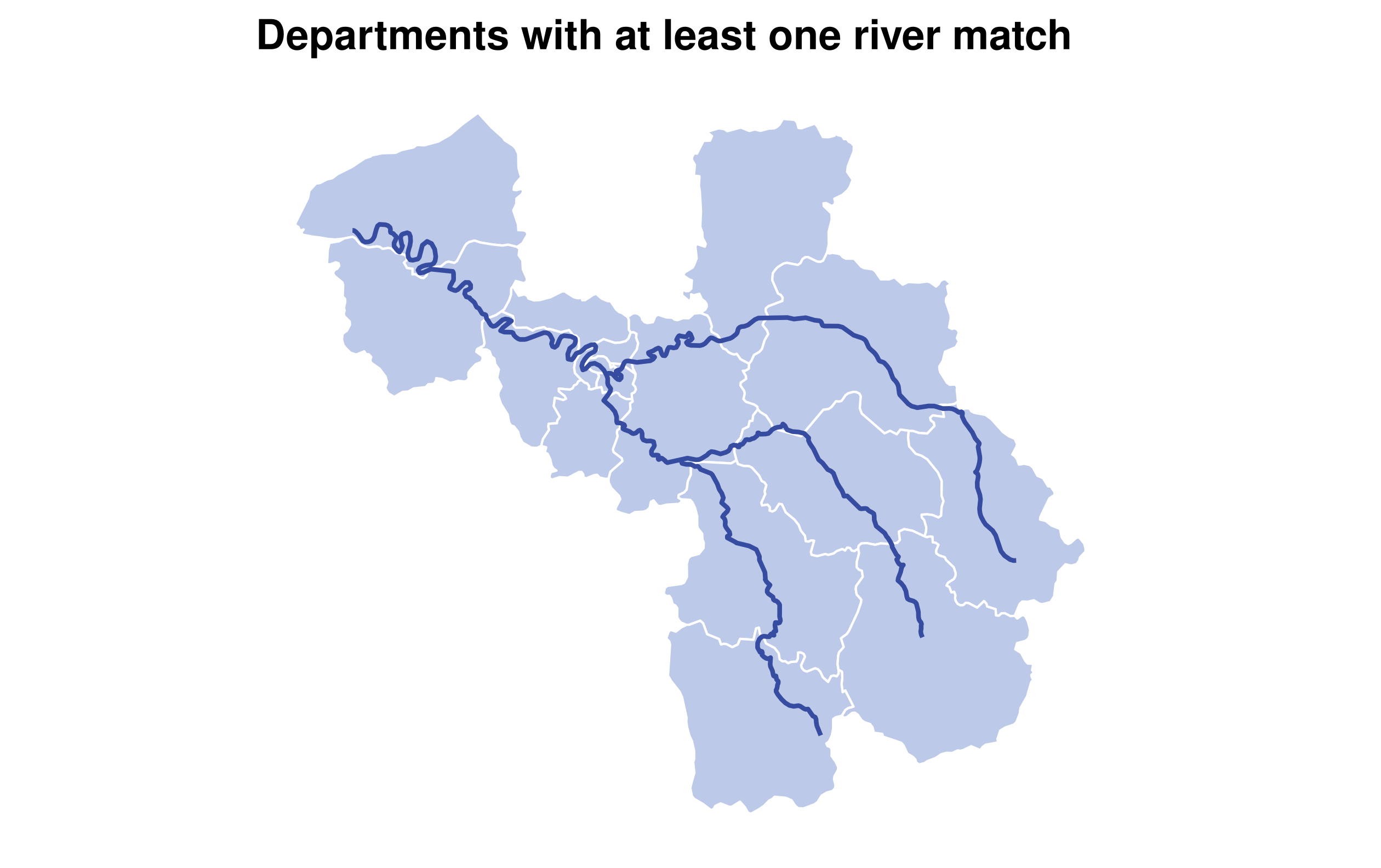
river_departments <- st_filter(france, seine)

nrow(river_departments)

## [1] 17

st_filter() uses st_intersects() by default.

• Keeps the full department geometry.
• Keeps the department attributes.
• Keeps each matching department once.

[Sources] - https://r-spatial.github.io/sf/reference/st_join.html

Filtering preserves whole polygons

Join when you need attributes from both layers

department_rivers <- st_join(france, seine, left = FALSE)

tibble(
  Output = c("Filtered departments", "Department–river matches"),
  Rows = c(nrow(river_departments), nrow(department_rivers))
) %>% knitr::kable()

Output	Rows
Filtered departments	17
Department–river matches	22

The join keeps the left-hand geometry and adds river attributes. A department appears once per matching river feature.

Check row counts after a spatial join, just as you would after an attribute join.

[Sources] - https://r-spatial.github.io/sf/reference/st_join.html left=FALSE discards departments with no match. The default left=TRUE would retain them with missing right-hand attributes.

Intersect when you need clipped geometry

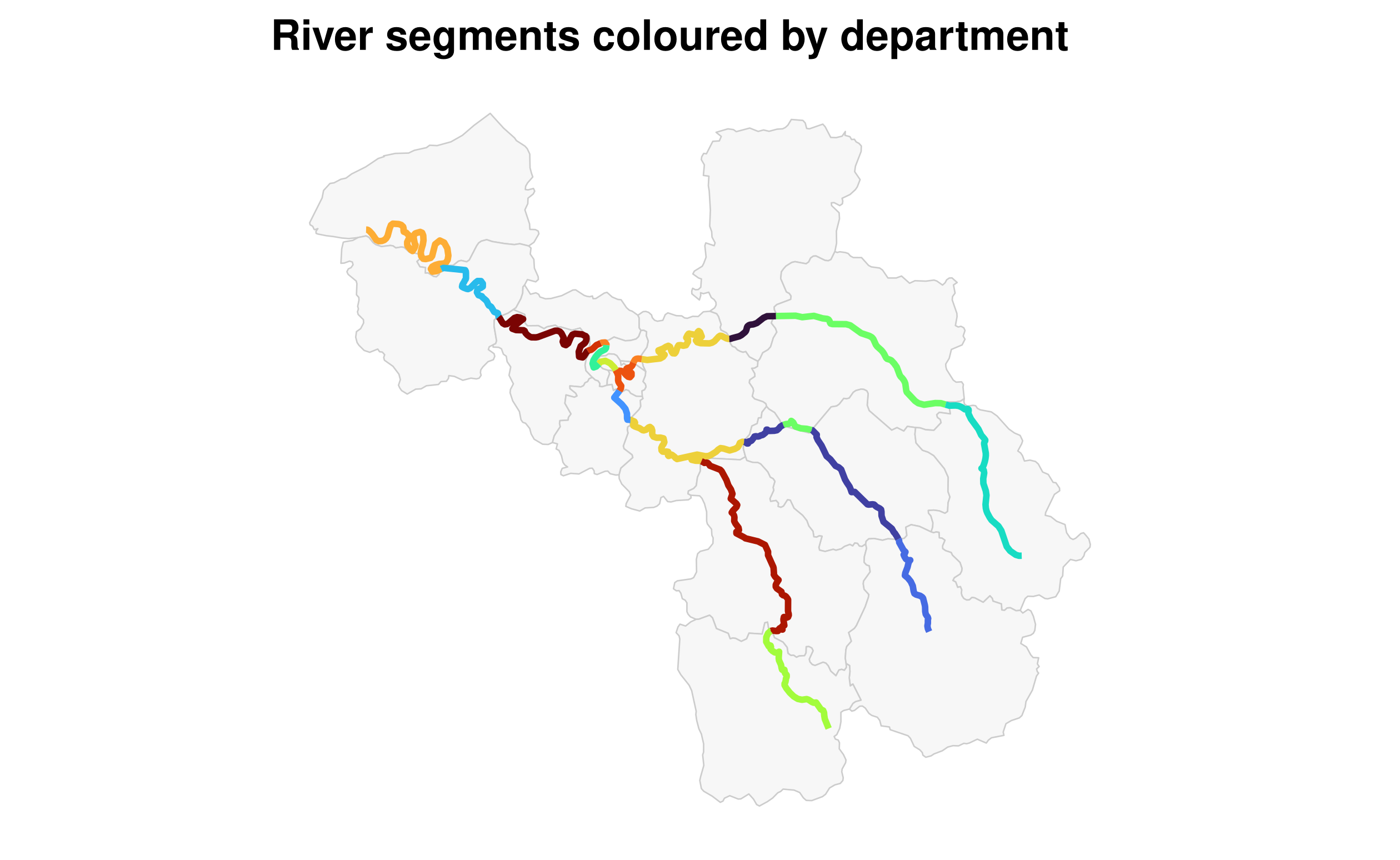
river_pieces <- st_intersection(
  france %>% select(ID),
  seine %>% select(name)
)

st_geometry_type(river_pieces) %>% as.character() %>% table()

## .
##      LINESTRING MULTILINESTRING 
##              21               1

A polygon intersected with a river line produces the part of the line inside the polygon, with attributes from both inputs.

[Sources] - https://r-spatial.github.io/sf/reference/geos_binary_ops.html Boundary-only contacts can produce points in some datasets; inspect geometry type instead of assuming every intersection has the same dimension.

Intersection divides rivers at boundaries

Colours identify department membership along the river; they do not encode a magnitude.

Choose the output you need

Task	Function	Geometry in the result
Identify matches	st_intersects()	None; returns matching indices
Keep matching departments	st_filter()	Original department polygons
Add river attributes	st_join()	Polygons; one per match
Clip rivers by department	st_intersection()	Overlapping river pieces

Ask two questions: Which rows should remain? What should their geometry represent?

Practice: choose a spatial operation

1. Keep villages within a study region.
2. Attach county names to village points.
3. Keep only the part of a road inside each county.
4. Find every county within 20 km of a river.

For each task, specify the left-hand unit, the spatial rule and whether geometry should change.

Possible answers: st_filter with st_within (decide boundary convention); st_join(points,counties); st_intersection(roads,counties); st_filter(counties,river,.predicate=st_is_within_distance,dist=20000) in an appropriate metre-based CRS. A buffer plus intersection/filter is another solution. Predicate choices depend on boundary inclusion.

Research examples

---

Use geometry without losing the meaning of the data

Read the village outcomes

load("data/china_map_dt.Rdata")
dt_plot %>% slice_head(n = 4) %>%
  knitr::kable(digits = c(0, 2, 2, 3, 0),
    col.names = c("ID", "Longitude", "Latitude", "Migration share", "Group"))

ID	Longitude	Latitude	Migration share	Group
2106	125.18	41.85	0.020	SPI only
2109	122.56	40.77	0.061	SPI only
2110	121.41	42.43	0.015	No Valid IV
2205	125.49	42.98	0.231	SPI only

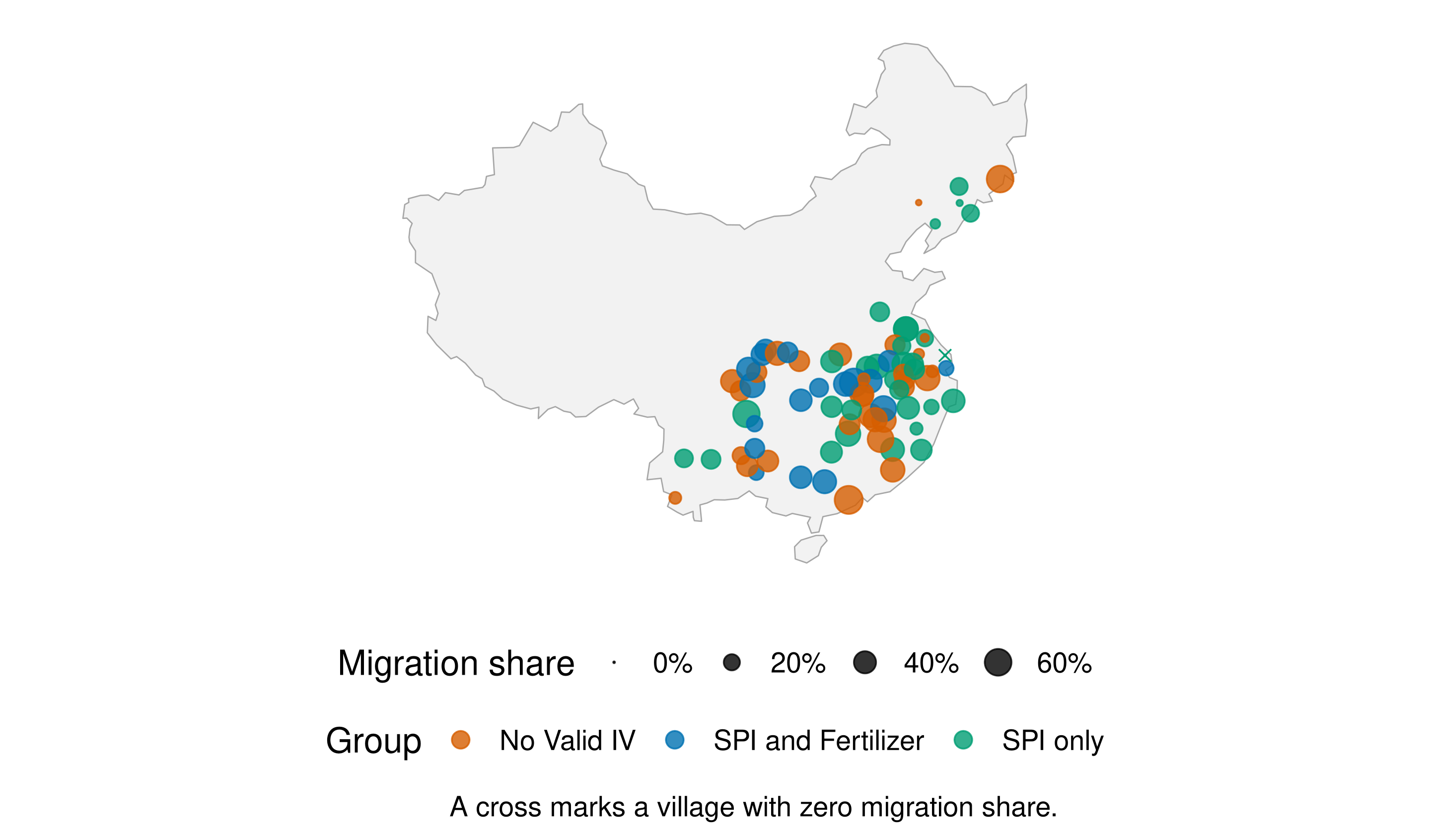
The supplied table contains 79 villages, coordinates, a migration share and model-based group labels.

[Sources] - Local course dataset: data/china_map_dt.Rdata - https://zhan-gao.github.io/files/zgao_gmm.pdf The notes connect the example to research on agricultural productivity, migration and instrument-validity classifications. The table itself does not document the survey year or denominator; do not infer either from the map.

Turn longitude and latitude into points

villages <- st_as_sf(dt_plot,
  coords = c("longitude", "latitude"),
  crs = 4326, remove = FALSE)

stopifnot(!anyDuplicated(villages$id))
range(villages$migrant_worker_ratio)

## [1] 0.0000000 0.6758242

This example assumes the supplied longitude/latitude use WGS84. Confirm that assumption with the data provider in an actual project.

Once points are sf features, they can be transformed together with the map.

Prepare the country outline and palette

world <- st_as_sf(rnaturalearthdata::countries110)
china <- world %>% filter(admin == "China")
china_crs <- "+proj=laea +lat_0=35 +lon_0=105 +datum=WGS84 +units=m"
group_colours <- c("No Valid IV" = "#D55E00",
  "SPI and Fertilizer" = "#0072B2", "SPI only" = "#009E73")

The country outline comes from the bundled Natural Earth layer. The projection is centred near the study area.

Map colour and size to different variables

china_plot <- ggplot() +
  geom_sf(data = china, fill = "grey95", colour = "grey65") +
  geom_sf(data = villages,
    aes(size = migrant_worker_ratio, colour = group), alpha = 0.8) +
  geom_sf(data = filter(villages, migrant_worker_ratio == 0),
    aes(colour = group), shape = 4, size = 2, show.legend = FALSE) +
  scale_size_area(max_size = 5, labels = scales::percent,
                  name = "Migration share") +
  scale_colour_manual(values = group_colours, name = "Group") +
  coord_sf(crs = china_crs, datum = NA) +
  labs(caption = "A cross marks a village with zero migration share.")

Village outcomes and model classifications

[Sources] - Local course dataset: data/china_map_dt.Rdata - https://www.naturalearthdata.com/about/terms-of-use/ The Natural Earth 1:110m country layer is a coarse reference map, not evidence about village location precision. A zero migration share has zero bubble area; an additional cross marks its location.

What does this map establish?

• Location: where the sampled villages are recorded.
• Size: the supplied migration share; a cross marks zero.
• Colour: the supplied group classification, not the strength of an effect.

Spatial patterns are descriptive. The map does not establish instrument validity, causality or national representativeness.

Check the survey year, rate denominator and coordinate source before using the figure as research evidence.

Audit county attributes before mapping

load("data/counties_treated.Rdata")
counties_treated %>%
  summarise(Rows = n(), `Missing FIPS` = sum(is.na(lock_fips)),
    `Dated Feb 1` = sum(first_treated_date == as.Date("2020-02-01"))) %>%
  knitr::kable()

Rows	Missing FIPS	Dated Feb 1
1927	50	1681

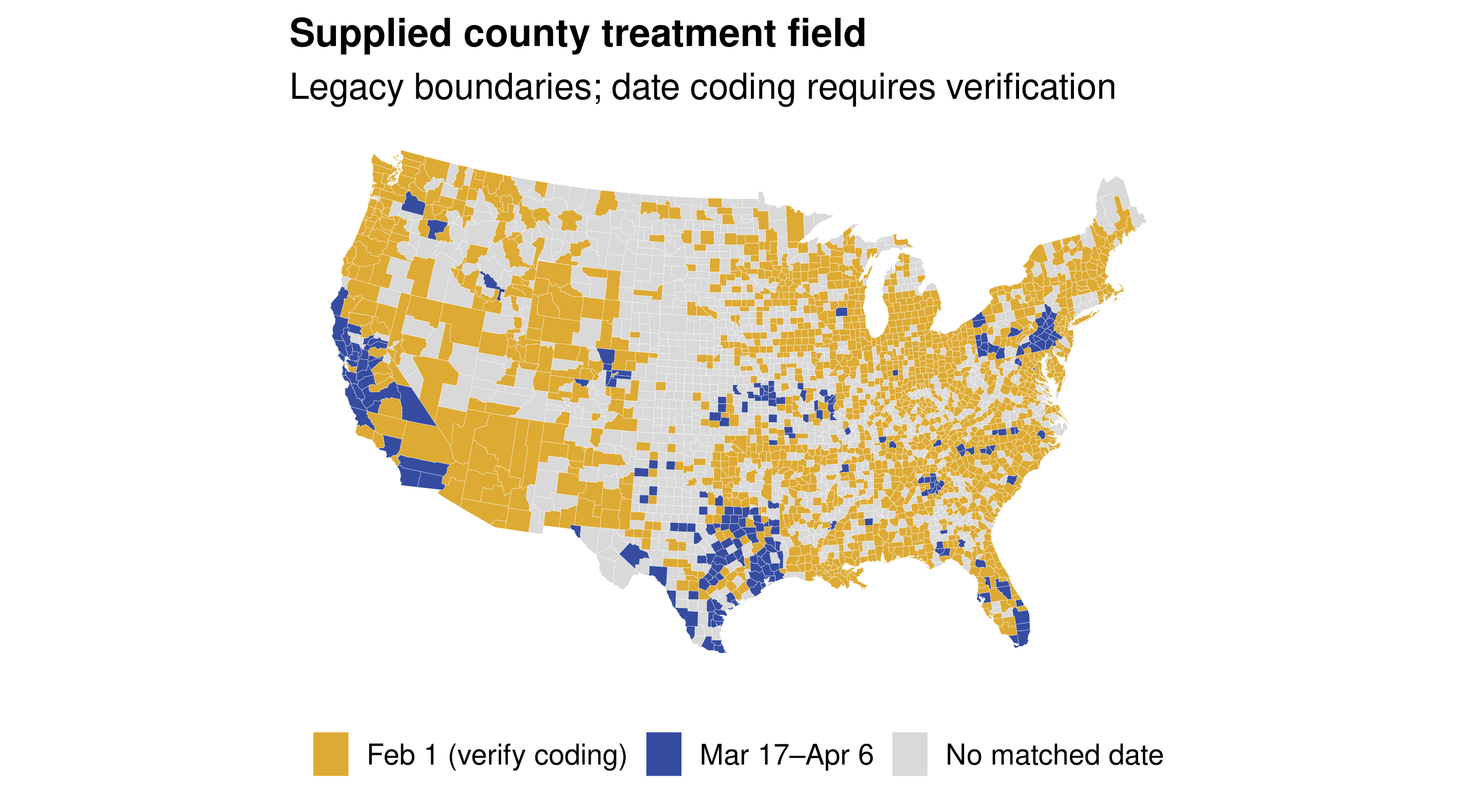
The notes use a field called first_treated_date. 1,681 rows share 2020-02-01, and 50 rows have no county identifier.

Treat this as a supplied treatment field to validate, not a verified calendar of county lockdown orders.

[Sources] - Local course dataset: data/counties_treated.Rdata There is no generating script or codebook for this field in the supplied material. Do not assume Feb 1 is a real order date or silently recode it as untreated.

Prepare a unique county key

county_dates <- counties_treated %>%
  filter(!is.na(lock_fips)) %>%
  mutate(FIPS = sprintf("%05d", lock_fips)) %>%
  select(FIPS, first_treated_date)

stopifnot(!anyDuplicated(county_dates$FIPS))
nrow(county_dates)

## [1] 1877

FIPS codes are identifiers: preserve the five-character form, including leading zeros.

The 50 records without county IDs cannot be matched to county polygons.

Give the boundary layer the same key

county_shapes <- maps::map("county", plot = FALSE, fill = TRUE) %>%
  st_as_sf()
county_lookup <- maps::county.fips %>%
  transmute(ID = sub(":.*$", "", polyname),
            FIPS = sprintf("%05d", fips)) %>% distinct()
stopifnot(!anyDuplicated(county_lookup$ID))
county_shapes <- county_shapes %>%
  left_join(county_lookup, by = "ID")
stopifnot(!anyNA(county_shapes$FIPS))

The bundled maps layer supplies legacy contiguous-U.S. county boundaries for this join demonstration.

Use a documented, matching boundary vintage for substantive analysis.

[Sources] - https://search.r-project.org/CRAN/refmans/maps/html/county.html - https://search.r-project.org/CRAN/refmans/maps/html/county.fips.html st_as_sf groups colon-suffixed polygon pieces into county features by default. Normalize the crosswalk names in the same way, then remove identical key pairs. The map package crosswalk matches polygon names to county FIPS. The 3,076 features correspond to 3,075 unique FIPS: Park County and Yellowstone National Park share code 30067 in this legacy lookup. This layer avoids a live boundary download while teaching an attribute join. The appendix shows tigris acquisition with an explicit year.

An attribute join keeps the map geometry

county_map <- county_shapes %>%
  left_join(county_dates, by = "FIPS", relationship = "many-to-one")
unmatched_dates <- county_dates %>%
  anti_join(st_drop_geometry(county_shapes), by = "FIPS")

tibble(Check = c("Boundary features", "Features after join",
                  "Date records without a boundary match"),
       Count = c(nrow(county_shapes), nrow(county_map),
                 nrow(unmatched_dates))) %>% knitr::kable()

Check	Count
Boundary features	3076
Features after join	3076
Date records without a boundary match	52

We match FIPS values, not spatial overlap. The geometry stays on the left.

Make unusual and missing values visible

county_map <- county_map %>%
  mutate(date_group = case_when(
    is.na(first_treated_date) ~ "No matched date",
    first_treated_date == as.Date("2020-02-01") ~ "Feb 1 (verify coding)",
    TRUE ~ "Mar 17–Apr 6"),
    date_group = factor(date_group, levels = c(
      "Feb 1 (verify coding)", "Mar 17–Apr 6", "No matched date")))

• Show the large February group explicitly while its meaning is unresolved.
• Keep unmatched records distinct from recorded dates.
• A missing match does not establish absence of treatment.

A map can expose a data-quality question

A reliable spatial workflow

1. Identify the observation unit and attribute definitions.
2. Inspect geometry, CRS and units.
3. Transform into a suitable CRS before the intended operation.
4. Choose an attribute join, spatial predicate or geometry operation.
5. Check matches, row counts, missing values and resulting geometry.
6. Design the map to support a clearly stated comparison.

A clean map is the final step of a checked data analysis.

Practice: build and audit a spatial result

Using the North Carolina data:

1. Compute county area in km² in EPSG:32119.
2. Keep counties with at least 5,000 births in BIR74.
3. Map them and dissolve their shared boundaries.
4. Explain the units and period represented by the threshold.

Extension: compute the minimum distance from each county to Durham. What result should Durham and its neighbours have?

Use nc_m, filter(BIR74 >= 5000), st_union(), and st_distance(nc_m, filter(nc_m, NAME == ‘Durham’)). Birth totals cover July 1974–June 1978. Durham and counties whose geometries touch Durham have zero minimum distance (up to numerical precision).

Resources

• Simple Features for R: data structures and spatial operations.
• Geocomputation with R: vector and raster workflows.
• Spatial Data Science: spatial data concepts and analysis.
• tidycensus: Census attributes and geometry.
• Leaflet for R: interactive maps.

Adapted in part from Grant McDermott’s EC607 spatial notes. The accompanying course notes provide additional context.

Projection and data-access examples

---

Additional tools for your own projects

Choose a projection for the comparison

Goal	Useful starting point	Limitation to check
Local geometry and distance	A suitable state-plane or UTM CRS	Area of use and distance distortion
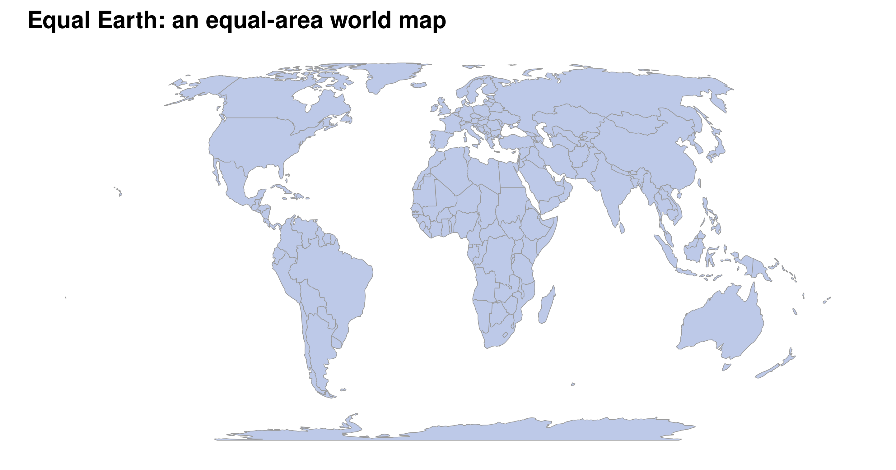
Compare country areas	Equal Earth, EPSG:8857	Shapes still change
Centre a regional map	Lambert azimuthal equal-area	Distortion grows away from the centre
Align with web tiles	Web Mercator, EPSG:3857	Strong area distortion at high latitudes

[Sources] - https://proj.org/en/stable/operations/projections/eqearth.html - https://proj.org/en/stable/operations/projections/laea.html - https://proj.org/en/stable/operations/projections/webmerc.html There is no universally best map projection. A CRS suitable for display is not automatically suitable for the intended measurement.

Global areas in Equal Earth

[Sources] - https://www.naturalearthdata.com/about/terms-of-use/ - https://proj.org/en/stable/operations/projections/eqearth.html

Change the display without changing the data

ggplot(world) +
  geom_sf(fill = "grey90", colour = "grey60", linewidth = 0.2) +
  coord_sf(crs = 8857)

# Transform the stored object instead:
world_equal_area <- st_transform(world, 8857)

If you see lines stretching across the map, inspect polygons near the map seam and the selected central meridian.

Changing the colour palette will not repair a geometry or projection problem.

Crop a study region explicitly

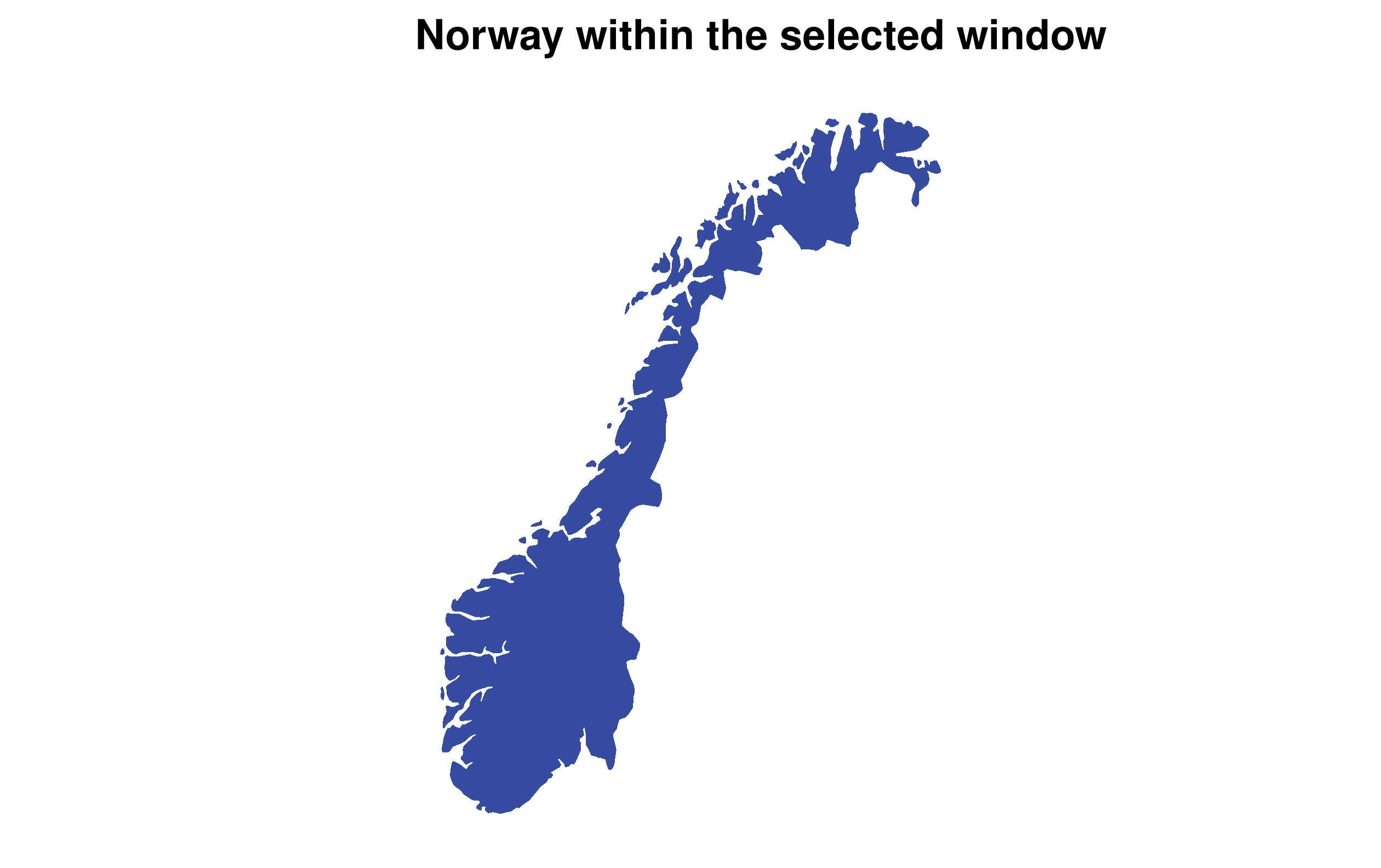
norway <- maps::map("world", "norway", plot = FALSE, fill = TRUE) %>%
  st_as_sf()
mainland_norway <- norway %>%
  st_crop(c(xmin = 4, xmax = 32, ymin = 57, ymax = 72))

st_crop() clips geometry to a bounding rectangle in the object’s current CRS.

This window removes northern island territories for a mainland-focused display. Cropping is a geographic selection, not a data-cleaning default.

A mainland-focused Norway map

[Sources] - https://r-spatial.github.io/sf/reference/st_crop.html - https://search.r-project.org/CRAN/refmans/maps/html/world.html EPSG:3035 is a Europe-centred equal-area CRS used here for a continental display. UTM zone 32N does not cover all of Norway equally well. The Faroe Islands are not Norwegian territory.

Set up Census access

Request a free Census API key, then run this once in your R console.

tidycensus::census_api_key("YOUR_KEY", install = TRUE)

• Restart R to load the saved key from .Renviron.
• Keep the key out of shared scripts and slides.
• Run the following optional recipes from lectures/; data/ refers to lectures/data/.

[Sources] - https://walker-data.com/tidycensus/reference/census_api_key.html [/Sources]

Download a fixed ACS sample

rent = tidycensus::get_acs(
  geography = "tract", variables = "B25064_001",
  state = c("WA", "OR"), year = 2023, survey = "acs5",
  geometry = TRUE, cb = TRUE, moe_level = 90
)
saveRDS(rent, "data/rent_acs5_2023.rds")

• The 2023 ACS five-year release covers 2019–2023.
• estimate is tract median monthly gross rent, in dollars; gross rent includes renter-paid utilities and fuels.
• moe gives the associated 90% margin of error; geometry stores tract boundaries.

The universe is renter-occupied housing units paying cash rent. B25064_001 is the detailed-table median gross rent variable; tidycensus returns the E estimate and M margin-of-error fields together. Five-year estimates are period estimates, not observations from the last year alone. The call uses generalized cartographic boundaries through tigris. It is deliberately unevaluated: the classroom deck does not call the live API.

[Sources] - https://api.census.gov/data/2023/acs/acs5/groups/B25064.html - https://walker-data.com/tidycensus/reference/get_acs.html - https://www.census.gov/newsroom/blogs/random-samplings/2017/12/rents.html [/Sources]

Save the metropolitan boundaries

Select Portland–Vancouver–Hillsboro, Corvallis, and Eugene–Springfield by their geographic IDs.

or_metros = tigris::core_based_statistical_areas(
  year = 2023, cb = TRUE
) |>
  filter(GEOID %in% c("38900", "18700", "21660")) |>
  select(metro_id = GEOID, metro_name = NAME)
saveRDS(or_metros, "data/or_metros_2023.rds")

The Portland metro crosses the Oregon–Washington border, so our tract download includes both states.

Core-based statistical areas include metropolitan and micropolitan areas. The three selected IDs correspond to metropolitan areas. Pinning the same boundary year helps comparisons, but generalized boundaries can still differ at edges. Preserve the acquired files and record the package versions with the analysis for reproducibility.

[Sources] - https://walkerke.r-universe.dev/tigris/doc/manual.html#core_based_statistical_areas - https://www.census.gov/programs-surveys/metro-micro.html [/Sources]

Map the saved rent estimates

Once the acquisition steps are complete, plotting reads the saved file.

rent = readRDS("data/rent_acs5_2023.rds")
ggplot(rent) +
  geom_sf(aes(fill = estimate), colour = NA) +
  coord_sf(crs = 5070, datum = NA) +
  scale_fill_viridis_c(
    name = "Monthly rent (USD)", na.value = "grey85"
  ) +
  labs(caption = "Source: 2019–2023 ACS, tract medians")

Gray areas have no available estimate. Read the estimate together with its margin of error.

This map describes median gross rent for each tract; it does not display individual rents or rental listings. A large polygon occupies more ink regardless of the number of households it contains. Numerical sentinels from the raw Census API must not be interpreted as rents; tidycensus handles the standard missing-value codes.

[Sources] - https://walker-data.com/tidycensus/reference/get_acs.html - https://ggplot2.tidyverse.org/reference/ggsf.html [/Sources]

Check the spatial match

or_metros = readRDS("data/or_metros_2023.rds") |>
  st_transform(5070) |> st_make_valid()
rent_proj = rent |> st_transform(5070) |> st_make_valid()
metro_rent = st_join(
  rent_proj, or_metros, join = st_within, left = FALSE
)
stopifnot(!anyDuplicated(metro_rent$GEOID))

• This rule retains tracts lying within a selected metro.
• Inspect boundary tracts: separately generalized polygons can create small mismatches.
• For official membership, use the corresponding county-to-metro crosswalk and tract county codes.

Do not replace the predicate with st_intersects without checking the result: touching boundaries can create multiple matches. Keeping a left join during investigation makes unmatched observations visible, but most Oregon/Washington tracts lie outside these three selected metros, so an unmatched row is not itself an error. A point-on-surface assignment is a useful mapping convention if explicitly described; it is not a substitute for official membership. The stopifnot check detects duplicate GEOIDs, but cannot establish that every intended tract was retained.

[Sources] - https://r-spatial.github.io/sf/reference/st_join.html - https://www.census.gov/programs-surveys/metro-micro/about/delineation-files.html [/Sources]

Compare distributions of tract medians

metro_rent |>
  filter(!is.na(estimate)) |>
  ggplot(aes(x = estimate)) +
  geom_histogram(binwidth = 100, boundary = 0) +
  facet_wrap(~metro_name, ncol = 1) +
  labs(x = "Tract median monthly gross rent (USD)",
       y = "Number of tracts")

Each tract contributes once. The histogram describes tract medians, not the distribution of household rents.

Treat differences cautiously when margins of error are large; averaging tract medians does not recover a metro median.

The histogram is an unweighted descriptive comparison across tracts. Tracts differ in their number of renter households and their estimation precision. Use the Census metro-level estimate when the question concerns the median for an entire metropolitan area.

[Sources] - https://walker-data.com/tidycensus/reference/get_acs.html - https://ggplot2.tidyverse.org/reference/geom_histogram.html [/Sources]

Explore an interactive map

nc_web = st_transform(nc, 4326)
leaflet::leaflet(nc_web) |>
  leaflet::addProviderTiles("CartoDB.Positron") |>
  leaflet::addPolygons(
    label = ~NAME, weight = 1,
    color = "#354CA1", fillOpacity = 0.2
  )

Pan and zoom to inspect counties; hover to see their names. The background tiles require an internet connection.

The recipe reuses the nc object from the main lecture. Transform sf features to WGS84 longitude/latitude before supplying them to Leaflet. The provider adds tile attribution automatically. An interactive map supports exploration; keep static maps for a fixed classroom comparison.

[Sources] - https://rstudio.github.io/leaflet/articles/shapes.html - https://rstudio.github.io/leaflet/reference/addProviderTiles.html [/Sources]

Install only the packages you need

install.packages(c("sf", "tidyverse", "maps",
                   "spData", "rnaturalearthdata"))
# Optional Census and interactive-map examples:
install.packages(c("tidycensus", "tigris", "leaflet"))
sf::sf_extSoftVersion()

• sf connects R to GDAL, GEOS, and PROJ; its units dependency uses UDUNITS-2.
• R package binaries usually include what is needed on Windows and macOS.
• Linux and source installations may require system development libraries; follow the sf installation guide.

These are optional console setup commands, not instructions executed while rendering. Core package choices should match the main deck’s setup; add rnaturalearth/rnaturalearthdata if the projection examples use those packages. The external library versions help explain numerical differences across machines. Linux system package names differ by distribution, so the slide links to maintained installation instructions rather than giving one universal command.

[Sources] - https://r-spatial.github.io/sf/#installing - https://r-quantities.github.io/units/ [/Sources]

Start with the unit and the spatial question

A village point, a county polygon and a clipped river segment represent different observations.

Choose the geometry and operation that match the question, then audit the result before interpreting the map.

Return to the spatial workflow