set.seed(123) # Please don't change this seed.

# You may load packages you plan to use (optional):
library(tidyverse)ECON 4354/6354 — Homework 1
- This homework is a coding assignment. Please follow the instructions to complete the tasks.
- Use Quarto/Knitr chunks for all work.
- Turn in the rendered HTML and your
.qmdsource via Canvas.
0. Setup
1. OLS Estimation
Recall that we implemented the OLS estimator in the lecture (link).
Please write a function ols_est(X, y) that implements the OLS estimator and returns both the estimate dcoefficients and the t-values.
# TODO: finish the function ols_est(X, y).

ols_est <- function(X, y, b0 = rep(0, ncol(X))) {
  # Get dimensions
  n <- nrow(X)
  k <- ncol(X)

  # OLS estimator
  bhat <- solve(t(X) %*% X, t(X) %*% y)

  # variance of residuals & vcov
  ehat <- y - X %*% bhat
  sigma2 <- as.numeric(crossprod(ehat) / (n - k))
  vcov <- sigma2 * solve(t(X) %*% X)
  se <- sqrt(diag(vcov))

  # t-values
  t_values <- (bhat - b0) / se

  return(list(bhat = bhat, se = se, t_values = t_values))
}
Please generate a simple test dataset to check if your function is working properly by comparing with the result from lm().
Tip
Use ?lm to see how to use lm() to run the linear regression.
# TODO: Test if ols_est() is working properly

# Generate a simple test dataset
n_test <- 100
X_test <- cbind(1, rnorm(n_test), rnorm(n_test)) # intercept + 2 regressors
beta_true <- c(1, 2, 3) # true coefficients
y_test <- X_test %*% beta_true + rnorm(n_test)

# Compare the result from ols_est() and lm()
# Using our function
result_ols <- ols_est(X_test, y_test)

# Using lm()
lm_result <- lm(y_test ~ X_test[, 2] + X_test[, 3])

# Compare coefficients
cat("Our OLS function coefficients:\n")
Our OLS function coefficients:print(result_ols$bhat) [,1]
[1,] 1.135065
[2,] 1.866828
[3,] 3.023811cat("\nlm() coefficients:\n")
lm() coefficients:print(coef(lm_result))(Intercept) X_test[, 2] X_test[, 3]
1.135065 1.866828 3.023811 # Compare standard errors
cat("\nOur OLS function standard errors:\n")
Our OLS function standard errors:print(result_ols$se)[1] 0.09614007 0.10486949 0.09899469cat("\nlm() standard errors:\n")
lm() standard errors:print(summary(lm_result)$coefficients[, 2])(Intercept) X_test[, 2] X_test[, 3]
0.09614007 0.10486949 0.09899469 # Compare t-values
cat("\nOur OLS function t-values:\n")
Our OLS function t-values:print(result_ols$t_values) [,1]
[1,] 11.80637
[2,] 17.80144
[3,] 30.54519cat("\nlm() t-values:\n")
lm() t-values:print(summary(lm_result)$coefficients[, 3])(Intercept) X_test[, 2] X_test[, 3]
11.80637 17.80144 30.54519 2. Monte Carlo Simulation
Let’s apply the skills learned in the class to implement a Monte Carlo simulation.
In such experiments, we sample data from a specified statistical model and examine the finite sample performance of estimation/inference procedures.
For different data generating processes, different primitive parameter values, and different sample sizes \(n\), we simulate data and estimate the model for many times and summarized the results (in most cases) by measures like (empirical) Bias, RMSE, size and empirical power functions, or empirical density plots, to examine the finite sample behavior of the estimation/inference procedures.
In this exercise, we will focus on the finite sample estimation accuracy of the OLS estimator in linear regression models. The accuracy can be measured by bias and root mean square error (RMSE).
Generically, bias and root mean square error (RMSE) are calculated by \[bias = R^{-1}\sum_{r=1}^R \left( \hat{ \theta}^{(r)} - \theta_0 \right),\] \[RMSE = \left(R^{-1}\sum_{r= 1}^R \left( \hat{\theta}^{(r)} -\theta_0 \right)^2\right)^{1/2},\] for true parameter \(\theta_0\) and its estimate \(\hat{\theta}^{(r)}\), and \(R\) is the number of replications.
Model
Consider a linear regression model \[y_i = \alpha + x_{i1}\beta_1 + x_{i2}\beta_2 + u_i\] for \(i = 1, 2, \ldots, n\), where \(n = 100\). \((y_i, x_i)\) are independently and identically distributed (i.i.d.) with \[u_i\sim i.i.d.N(0,1), \quad (x_{i1}, x_{i2})^\prime \sim i.i.d. N\left(\begin{pmatrix}0 \\ 1 \end{pmatrix}, \begin{pmatrix} \sigma_1^2 & \rho\sigma_1\sigma_2 \\ \rho\sigma_1\sigma_2 & \sigma_2^2 \end{pmatrix} \right).\] True parameters are \(a = 0.11\), \(\beta = (0.22, 0.33)^\prime\), \(\rho = 0.5\), \(\sigma_1 = 1\), and \(\sigma_2 = 4\).
Step 1: Data generating function
Pleaes write a function dgp(...) that takes the sample size \(n\) and model parameters as inputs and returns the simulated data \((y_i, x_{i1}, x_{i2})\) for \(i = 1, 2, \ldots, n\).
# TODO: simulate data
dgp <- function(n, alpha = 0.11, beta1 = 0.22, beta2 = 0.33,
                rho = 0.5, sigma1 = 1, sigma2 = 4) {
  # Generate correlated regressors (x1, x2)
  # Mean vector
  mu_x <- c(0, 1)

  # Covariance matrix
  Sigma_x <- matrix(
    c(
      sigma1^2, rho * sigma1 * sigma2,
      rho * sigma1 * sigma2, sigma2^2
    ),
    nrow = 2, ncol = 2
  )

  # Generate (x1, x2) from bivariate normal
  X_reg <- MASS::mvrnorm(n, mu = mu_x, Sigma = Sigma_x)
  x1 <- X_reg[, 1]
  x2 <- X_reg[, 2]

  # Generate error term
  u <- rnorm(n, mean = 0, sd = 1)

  # Generate dependent variable
  y <- alpha + beta1 * x1 + beta2 * x2 + u

  # Return data as data frame
  return(data.frame(y = y, x1 = x1, x2 = x2))
}
Step 2: Setup Primitive Parameters
# TODO: setup primitive parameters: sample size, true parameters, etc.

# Simulation parameters
n <- 100 # sample size
R <- 1000 # number of replications

# True parameters
alpha_true <- 0.11
beta1_true <- 0.22
beta2_true <- 0.33
rho_true <- 0.5
sigma1_true <- 1
sigma2_true <- 4

# True parameter vector
theta_true <- c(alpha_true, beta1_true, beta2_true)
Step 3: Run Simulation
# TODO: Run the simulation (generate data - estimation - save results) for 1000 replications

# Initialize storage for results
results <- matrix(NA, nrow = R, ncol = 3) # 3 coefficients: alpha, beta1, beta2
colnames(results) <- c("alpha", "beta1", "beta2")

# Run simulation
for (r in 1:R) {
  # Generate data
  data <- dgp(
    n = n, alpha = alpha_true, beta1 = beta1_true, beta2 = beta2_true,
    rho = rho_true, sigma1 = sigma1_true, sigma2 = sigma2_true
  )

  # Create design matrix (intercept + x1 + x2)
  X <- cbind(1, data$x1, data$x2)

  # Estimate using our OLS function
  ols_result <- ols_est(X, data$y)

  # Store results
  results[r, ] <- ols_result$bhat
}

# Display first few results
head(results)
alpha beta1 beta2
[1,] 0.03398565 -0.006976698 0.3403150
[2,] 0.21648747 0.216686199 0.2974552
[3,] 0.10526201 0.173595952 0.3090265
[4,] 0.23749991 0.149111058 0.2984990
[5,] 0.18249103 0.257914065 0.2959098
[6,] 0.01348023 0.359885326 0.3158113Step 4: Summarize Results
# TODO: Write a function to calculate bias and RMSE
sum_results <- function(estimates, true_params, param_names = NULL) {
  # Calculate bias
  bias <- colMeans(estimates) - true_params

  # Calculate RMSE
  rmse <- sqrt(colMeans((estimates - matrix(true_params,
    nrow = nrow(estimates),
    ncol = ncol(estimates), byrow = TRUE
  ))^2))

  # Set parameter names if not provided
  if (is.null(param_names)) {
    if (length(true_params) == 3) {
      param_names <- c("alpha", "beta1", "beta2")
    } else if (length(true_params) == 2) {
      param_names <- c("alpha", "beta1")
    } else {
      param_names <- paste0("param", 1:length(true_params))
    }
  }

  # Create summary table
  summary_table <- data.frame(
    Parameter = param_names,
    True_Value = true_params,
    Mean_Estimate = colMeans(estimates),
    Bias = bias,
    RMSE = rmse
  )

  return(summary_table)
}

# TODO: Summarize and report the bias and RMSE
summary_results <- sum_results(results, theta_true)
print(summary_results)
Parameter True_Value Mean_Estimate Bias RMSE
alpha alpha 0.11 0.1155052 0.0055051758 0.10318576
beta1 beta1 0.22 0.2189192 -0.0010808443 0.11911991
beta2 beta2 0.33 0.3298367 -0.0001633363 0.03010833# TODO: plot the empirical density of the estimated coefficient beta_1 across replications
library(ggplot2)
# Plot empirical density of beta1
ggplot(data.frame(beta1 = results[, "beta1"]), aes(x = beta1)) +
geom_density(fill = "blue", alpha = 0.3) +
geom_vline(xintercept = beta1_true, color = "red", linetype = "dashed", size = 1) +
labs(
title = "Empirical Density of Estimated Beta1",
x = "Beta1 Estimates",
y = "Density"
) +
theme_minimal()Warning: Using `size` aesthetic for lines was deprecated in ggplot2 3.4.0.
ℹ Please use `linewidth` instead.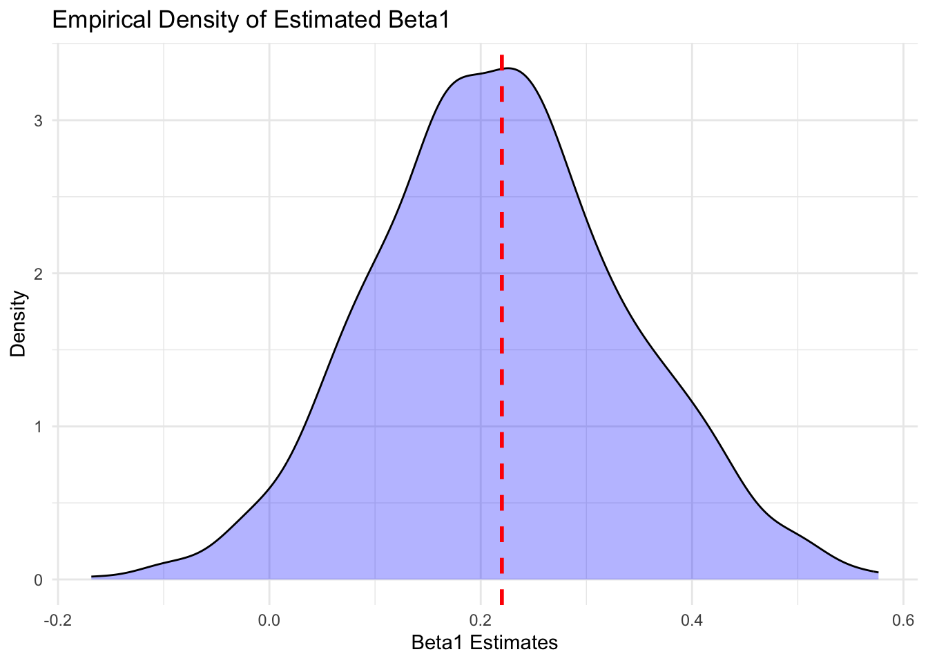
Step 5: Interpret your results
Please interpret your results and discuss the findings.
Step 6: Run simulation with different sample sizes
Let’s investigate how the estimation accuracy of the OLS estimator changes as the sample size increases.
# TODO: Run the simulation with different sample sizes
sample_sizes <- c(100, 200, 500, 1000)

# Initialize storage for results across different sample sizes
results_different_n <- list()

# Run simulation for each sample size
for (n_size in sample_sizes) {
  cat("Running simulation for n =", n_size, "\n")

  # Initialize storage for this sample size
  results_n <- matrix(NA, nrow = R, ncol = 3)
  colnames(results_n) <- c("alpha", "beta1", "beta2")

  # Run simulation
  for (r in 1:R) {
    # Generate data
    data <- dgp(
      n = n_size, alpha = alpha_true, beta1 = beta1_true, beta2 = beta2_true,
      rho = rho_true, sigma1 = sigma1_true, sigma2 = sigma2_true
    )

    # Create design matrix
    X <- cbind(1, data$x1, data$x2)

    # Estimate using our OLS function
    ols_result <- ols_est(X, data$y)

    # Store results
    results_n[r, ] <- ols_result$bhat
  }

  # Store results for this sample size
  results_different_n[[paste0("n_", n_size)]] <- results_n
}
Running simulation for n = 100
Running simulation for n = 200
Running simulation for n = 500
Running simulation for n = 1000 # Calculate summary statistics for each sample size
summary_different_n <- data.frame()
for (n_size in sample_sizes) {
results_n <- results_different_n[[paste0("n_", n_size)]]
summary_n <- sum_results(results_n, theta_true)
summary_n$Sample_Size <- n_size
summary_different_n <- rbind(summary_different_n, summary_n)
}
# Display results
print(summary_different_n) Parameter True_Value Mean_Estimate Bias RMSE Sample_Size
alpha alpha 0.11 0.1100650 6.498956e-05 0.105020161 100
beta1 beta1 0.22 0.2221331 2.133121e-03 0.118942460 100
beta2 beta2 0.33 0.3302845 2.844631e-04 0.029250235 100
alpha1 alpha 0.11 0.1070141 -2.985912e-03 0.072413381 200
beta11 beta1 0.22 0.2215646 1.564638e-03 0.083477945 200
beta21 beta2 0.33 0.3304110 4.110027e-04 0.019857969 200
alpha2 alpha 0.11 0.1086414 -1.358620e-03 0.048155575 500
beta12 beta1 0.22 0.2179149 -2.085071e-03 0.050595154 500
beta22 beta2 0.33 0.3301787 1.787083e-04 0.012475377 500
alpha3 alpha 0.11 0.1100217 2.165969e-05 0.033924343 1000
beta13 beta1 0.22 0.2175470 -2.452983e-03 0.036860677 1000
beta23 beta2 0.33 0.3303540 3.539533e-04 0.009377108 1000# Plot RMSE vs sample size for beta1
rmse_beta1 <- summary_different_n[summary_different_n$Parameter == "beta1", c("Sample_Size", "RMSE")]
ggplot(rmse_beta1, aes(x = Sample_Size, y = RMSE)) +
geom_line() +
geom_point() +
labs(
title = "RMSE of Beta1 vs Sample Size",
x = "Sample Size",
y = "RMSE"
) +
theme_minimal()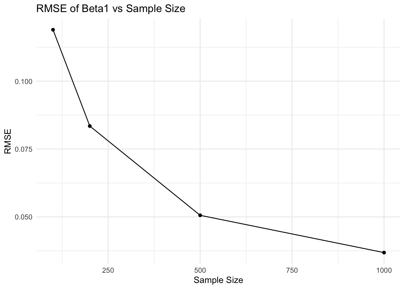
What do you observe? Why?
Step 7: Run simulation with misspecified model
Now, we re-do the simulation with the same data generating process.
However, when we run the regression, we only include the first regressor \(x_{i1}\) and the intercept while omitting the second regressor \(x_{i2}\).
# TODO: Run the simulation with misspecified model
# Initialize storage for misspecified model results
results_misspecified <- matrix(NA, nrow = R, ncol = 2) # Only intercept and beta1
colnames(results_misspecified) <- c("alpha", "beta1")

# Run simulation with misspecified model (omit x2)
for (r in 1:R) {
  # Generate data (same as before)
  data <- dgp(
    n = n, alpha = alpha_true, beta1 = beta1_true, beta2 = beta2_true,
    rho = rho_true, sigma1 = sigma1_true, sigma2 = sigma2_true
  )

  # Create design matrix with only intercept and x1 (omit x2)
  X_misspecified <- cbind(1, data$x1)

  # Estimate using our OLS function
  ols_result_misspecified <- ols_est(X_misspecified, data$y)

  # Store results (only alpha and beta1)
  results_misspecified[r, ] <- ols_result_misspecified$bhat
}

# Display first few results
head(results_misspecified)
alpha beta1
[1,] 0.4643403 0.7066507
[2,] 0.4454095 0.8423814
[3,] 0.3752038 0.8597395
[4,] 0.3811730 1.0935918
[5,] 0.5252322 0.8126518
[6,] 0.5111212 0.7610173# TODO: Check the bias and RMSE for beta_1 with the misspecified model
# True parameters for misspecified model (what we're actually estimating)
theta_misspecified_true <- c(alpha_true, beta1_true)
# Calculate summary for misspecified model
summary_misspecified <- sum_results(results_misspecified, theta_misspecified_true,
param_names = c("alpha", "beta1")
)
print("Misspecified Model Results:")[1] "Misspecified Model Results:"print(summary_misspecified) Parameter True_Value Mean_Estimate Bias RMSE
alpha alpha 0.11 0.4339357 0.3239357 0.3580699
beta1 beta1 0.22 0.8802508 0.6602508 0.6767678# Compare with correctly specified model for beta1
summary_correct <- sum_results(results, theta_true)
beta1_correct <- summary_correct[summary_correct$Parameter == "beta1", ]
beta1_misspecified <- summary_misspecified[summary_misspecified$Parameter == "beta1", ]
cat("\nComparison for Beta1:\n")
Comparison for Beta1:cat("Correctly specified model:\n")Correctly specified model:cat(" Bias:", beta1_correct$Bias, "\n") Bias: -0.001080844 cat(" RMSE:", beta1_correct$RMSE, "\n") RMSE: 0.1191199 cat("Misspecified model:\n")Misspecified model:cat(" Bias:", beta1_misspecified$Bias, "\n") Bias: 0.6602508 cat(" RMSE:", beta1_misspecified$RMSE, "\n") RMSE: 0.6767678 # Plot comparison of beta1 estimates
library(ggplot2)
comparison_data <- data.frame(
Model = rep(c("Correct", "Misspecified"), each = R),
Beta1 = c(results[, "beta1"], results_misspecified[, "beta1"])
)
ggplot(comparison_data, aes(x = Beta1, fill = Model)) +
geom_density(alpha = 0.5) +
geom_vline(xintercept = beta1_true, color = "red", linetype = "dashed", size = 1) +
labs(
title = "Comparison of Beta1 Estimates: Correct vs Misspecified Model",
x = "Beta1 Estimates",
y = "Density"
) +
theme_minimal()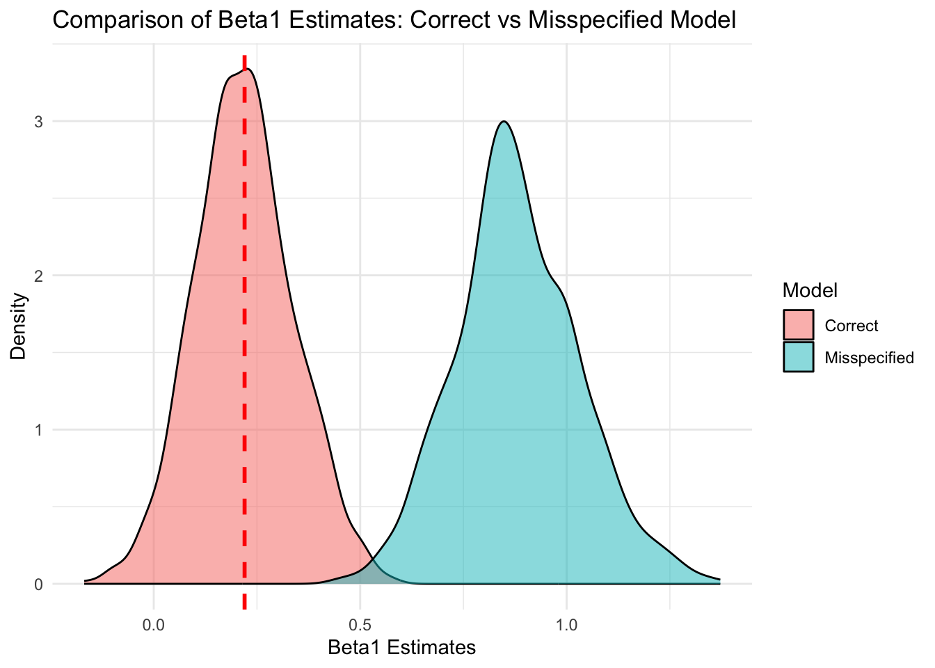
What do you observe? Why?
The estimates of the misspecified model are biased and have a larger RMSE than the correctly specified model, which demonstrates the omitted variable bias.