ECON 4370 / 6370 Computing for Economics

Lecture 15: Causal Inference

Zhan Gao

08 October 2026

Do cell phones fight crime?

• Regress state murder rates on cell-phone subscriptions, with state effects, a linear trend and eight controls. The coefficient is -0.37 with a t statistic of -5.4: cell phones “reduce” murder, and by more than legalized abortion does in the same regression.
• Nobody believes it. The regression that produced it is the one a famous paper used for abortion. What did it actually find, and how do we tell? Section 4.

The coefficient on the abortion rate in the same specification is minus 0.21 with t of minus 5.1 (Donohue and Levitt 2001, as replicated in Taddy’s Business Data Science). The cell-phone series is a placebo treatment: a variable with the same trend and no plausible effect on murder. Both pick up the one thing a linear trend cannot absorb, a quadratic trend. The deck returns to this slide after the double lasso.

Today’s route

1. Correlation, causation and counterfactuals: what a regression coefficient has meant so far, and what question a causal effect answers.
2. The potential outcomes framework: Y = g(D, \varepsilon), selection bias as omitted-variable bias, and when a difference in means is an average treatment effect.
3. Randomized experiments: the Oregon Health Insurance Experiment, noncompliance, and conditional average treatment effects.
4. Controlling for covariates: abortion and crime, placebo tests, and the double lasso.
5. Heterogeneous effects with trees and forests: the transformed outcome and the National Supported Work data.
6. Honest trees and post-selection inference: why intervals after model selection are too narrow, and sample splitting as the cure.

Additional derivations and code follow the main lesson.

Lectures 11 to 14 estimated E[Y | X] and judged the estimate out of sample. Today the target changes: what would Y be if we changed D, holding everything else fixed? That is a different quantity, and the machinery of the last four lectures (lasso, trees, forests, cross-validation) has to be modified before it can estimate it. Sections 1 to 4 fit one 80-minute session and sections 5 and 6 a second if the material is split across the two causal sessions of the schedule.

Packages and data

Run the examples from the lectures/ directory.

library(tidyverse)
library(glmnet)    # the lasso, for the double lasso in section 4
library(tree)      # regression trees, for sections 5 and 6
library(ranger)    # random forests, for section 5
library(foreign)   # read.dta() reads the Stata files of the Oregon experiment

File	Role
data/oregon_data/oregonhie_*.dta	The Oregon Health Insurance Experiment: lottery status, enrolment, and the 12-month survey
data/abortion.dat, data/us_cellphone.csv	Crime, abortion and controls by state and year, 1985 to 1997; US cell-phone subscriptions
data/dw_experimental_data.csv	The National Supported Work demonstration, 445 participants of a 1970s job training experiment

[Sources] - The Oregon data are the public-use files of Finkelstein et al. (2012), downloaded from the NBER; the cleaning code is in the appendix. - The abortion and cell-phone data accompany Taddy, Business Data Science (2019), chapter 6, and come from Donohue and Levitt (2001). - The NSW file is the Dehejia and Wahba (1999) experimental subsample of LaLonde (1986).

Correlation, causation and counterfactuals

---

What a regression coefficient has meant so far

• Every \hat\beta in this course has been a correlation: the association between a regressor and Y in the data we had.
• That is enough for two purposes: describing patterns in past data, and predicting future outcomes with \hat{\mathbf{E}}[Y \mid X = x] = G(x'\hat\beta), provided the process that generates the future is the one that generated the past.
• Often we need a prediction precisely because the process will change, usually because of something we do.

A firm changes its pricing or marketing after analysing past data. Consumers then respond to the new policy, not to the old mix of prices and promotions that produced the data. The coefficient from the past need not describe what happens next.

This is the sentence we kept repeating in lectures 8 to 14: “the coefficient is an association”. Today’s question is what extra assumption turns an association into an answer to a “what if” question, and what to do when the assumption fails.

Counterfactual prediction

• Forecasting after an intervention is counterfactual prediction: imagining how the system would respond if we changed one thing and held the rest fixed.
• A causal effect is defined relative to a counterfactual. Stating it forces us to say what we mean.

“What is the causal effect of cholesterol on heart attacks?” We cannot dial cholesterol up and down. Each concrete intervention is a different counterfactual, and each may have a different effect:

• prescribing cholesterol medication;
• changing diet;
• changing exercise.

• The counterfactual can be a policy we might actually run or a thought experiment for scientific understanding. Either way, be concrete about it.
• A clear counterfactual also tells us which made-up objects (utility, “true” preferences, behavioural stories) our model needs and which it can leave out.

Example of the last point: a demand model where consumers may be “tricked” by advertising. If the counterfactual is a tax change and we want tax revenue, the behavioural story may not matter. If the counterfactual is a policy that informs consumers, or the question is welfare, it does.

Lending, revisited

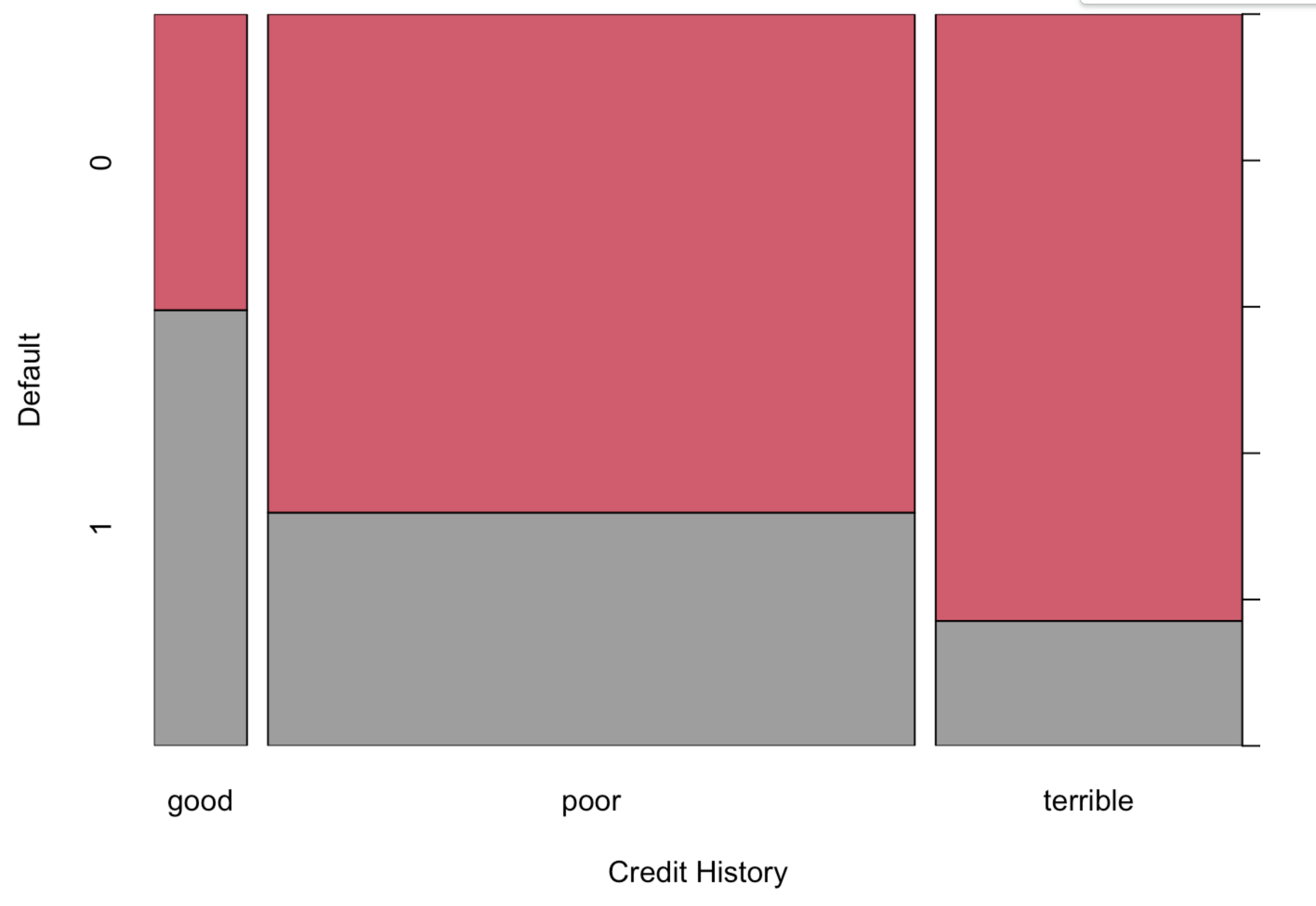
• In the logit of lecture 9, borrowers with better credit histories defaulted more often.
• Should the bank prefer borrowers with bad histories? No: those with good histories were approved for riskier loans, and the risk came with the loan.
• One counterfactual: tighten screening to require a better history, holding the loan type fixed. Under that policy, a better history should lower defaults.
• The correlation is biased for this effect. Two names for one problem: selection bias (good histories were selected into risky loans) or omitted-variable bias (the loan type is missing from the regression).

Other counterfactuals that “manipulate credit history” (a personal finance class, a mailing list of good-history consumers, a law forcing approval above a threshold) would have different effects. The counterfactual disciplines the question.

The figure is the mosaic plot of default against credit history from the German credit data of lecture 9. The point to land: “causal effect of credit history” is not one number until we say what intervention changes credit history and what is held fixed.

The potential outcomes framework

---

Does health insurance improve health?

• The US spends a larger share of GDP on health care than other rich countries and has worse outcomes. Would outcomes improve under universal coverage?
• That is a causal question: does having insurance raise health?
• In survey data, insured people are healthier. A causal story: insurance buys preventive care and early treatment.

Warning

A selection story: people with insurance also have higher incomes, steadier jobs and different backgrounds, all of which affect health directly. The comparison of insured and uninsured mixes the effect of insurance with the effect of being the kind of person who has it.

We now write this down in symbols. The framework is the same as the textbook linear model with different notation, and the notation is the point: it makes “holding everything else fixed” precise.

Ask the class for both stories before showing the callout. The rest of the section formalizes the selection story; section 3 uses an experiment in which insurance was assigned by lottery.

Potential outcomes

Let Y be the outcome (health) and D \in \{0, 1\} the treatment (D = 1: has insurance). Outcomes are determined by Y = g(D, \varepsilon), where g is an unknown function and \varepsilon collects every other factor that affects Y: income, job, background, luck.

• Fix a unit’s \varepsilon and imagine switching D. The two values g(0, \varepsilon) and g(1, \varepsilon) are the potential outcomes: health without insurance and health with it, everything else held fixed.
• The unit-level treatment effect is g(1, \varepsilon) - g(0, \varepsilon). It is causal because D is the only thing that changed.
• We observe Y = g(D, \varepsilon): one potential outcome per unit. The other is counterfactual.

Unit	D_i	g(0, \varepsilon_i)	g(1, \varepsilon_i)	Y_i	Effect
1	1	?	0.8	0.8	?
2	0	0.5	?	0.5	?
3	1	?	0.6	0.6	?

No unit-level effect is ever observed. Everything that follows is about estimating averages of them.

Three equivalent notations are in circulation: g(D, epsilon) as here, Y*(d) for the potential outcomes, or Y(0), Y(1). The appendix has a note on why some people prefer one over another; for estimation they lead to the same estimators.

The linear, homogeneous case

You know the special case where g is linear and additive in \varepsilon: g(D, \varepsilon) = \alpha + \beta D + \varepsilon, \qquad g(1, \varepsilon) - g(0, \varepsilon) = \beta \ \text{ for every } \varepsilon. The treatment effect is homogeneous: the same number for everyone.

When does OLS of Y on D recover \beta? With n observations, \hat\beta = \frac{\widehat{\operatorname{Cov}}(Y, D)}{\widehat{\operatorname{Var}}(D)} \approx \frac{\operatorname{Cov}(\alpha + \beta D + \varepsilon, D)}{\operatorname{Var}(D)} = \beta + \frac{\operatorname{Cov}(\varepsilon, D)}{\operatorname{Var}(D)}.

OLS recovers the causal effect when \operatorname{Cov}(\varepsilon, D) = 0: when the treatment is uncorrelated with everything else that matters for the outcome. The second term is the selection bias.

This is the introductory econometrics result in new clothes. The new clothes matter when we drop linearity on the next slides: independence of D and epsilon, rather than zero correlation, will be the assumption, and the difference in means, rather than a slope, the estimator.

Selection bias is omitted-variable bias

Can we expect \operatorname{Cov}(\varepsilon, D) = 0 in data on insurance and health? Only if the counterfactual says so: \varepsilon is everything held fixed in the counterfactual.

• \varepsilon includes income, job status and social background, which affect health directly, so they are part of g(0, \varepsilon) and g(1, \varepsilon).
• The same things are correlated with having insurance, so \operatorname{Cov}(\varepsilon, D) \neq 0.

Selection bias. People select into D = 1 or D = 0 on the basis of their \varepsilon.

Omitted-variable bias. Income, job and background should have been in the regression so that they are held fixed. Section 3 does that.

The orange juice and lending examples are the same story with D = price or credit history and \varepsilon = promotions or loan type.

The two phrases describe the same covariance from two sides. “Selection” describes how the data were generated; “omitted variable” describes what the regression lacks. Both tell us what a fix must do: break the covariance (an experiment) or condition on the variable (controls).

A simulation of selection bias

set.seed(0); n <- 5000
income <- rnorm(n)                                  # part of epsilon: affects health directly
y0 <- 1 + income + rnorm(n); y1 <- y0 + 0.5         # potential outcomes: the effect is 0.5 for everyone
D_obs <- as.numeric(income + rnorm(n) > 0)          # richer people are more likely to be insured
D_rct <- rbinom(n, 1, 0.5)                          # a lottery ignores income
Y_obs <- ifelse(D_obs == 1, y1, y0); Y_rct <- ifelse(D_rct == 1, y1, y0)
estimates <- c(observational = unname(coef(lm(Y_obs ~ D_obs))[2]),
               control_for_income = unname(coef(lm(Y_obs ~ D_obs + income))[2]),
               randomized = unname(coef(lm(Y_rct ~ D_rct))[2]))
round(estimates, 3)

##      observational control_for_income         randomized 
##              1.614              0.463              0.560

• The observational regression triples the true effect: \operatorname{Cov}(\varepsilon, D) / \operatorname{Var}(D) is about 1.11 here.
• Controlling for the part of \varepsilon that drives selection removes the bias. So does a lottery, without knowing what drives selection.

Both fixes appear in section 3: randomization (Oregon) and conditioning on the selection variable (household size). The simulation makes the point that the bias is not small or subtle: it can dominate the effect.

Prediction and causal prediction are different targets

Prediction (lectures 11 to 14)

• Write Y_i = f(X_i) + U_i with \mathbf{E}[U_i \mid X_i] = 0 by definition of f.
• The future looks like the past, as cross-validation assumes.
• The selection term \operatorname{Cov}(\varepsilon, D)/\operatorname{Var}(D) helps: it is one more way D carries information about Y.

Causal prediction (today)

• Y_i = g(D_i, \varepsilon_i), and \varepsilon_i is whatever the counterfactual holds fixed. In general f \neq g and U \neq \varepsilon.
• Intervening on D changes the relationship between D and \varepsilon; the past covariance no longer describes the future.
• The selection term hurts: we want \beta alone.

Pricing. To forecast demand after a price cut on its own, we want \beta. To forecast demand when price moves together with the promotions and advertising that always moved with it in the data, we want \beta plus the selection term, and ordinary prediction is right.

This slide is why causal inference is not just “prediction done carefully”. The two targets differ by the selection term, and which one is wanted depends on what will change. The out-of-sample machinery of earlier lectures validates the first target only.

Heterogeneous treatment effects

Linear and additive g forces the same effect \beta on everyone. That is rarely plausible: the effect of insurance on health should differ by

• baseline health (the healthy never use the insurance),
• wealth (the wealthy pay out of pocket anyway).

Models with heterogeneous effects are not additively separable in \varepsilon:

• random coefficients, Y = \alpha + (\beta + \varepsilon_1) D + \varepsilon_2, with unit-level effect \beta + \varepsilon_1;
• the random-utility logit, Y = \mathbf{1}(\alpha + \beta D \geq \varepsilon), with unit-level effect in \{-1, 0, 1\}.

There is no single \beta to recover. The natural target is the average treatment effect, \text{ATE} = \mathbf{E}[g(1, \varepsilon) - g(0, \varepsilon)], the population average of the unit-level effects. Later, averages within groups defined by covariates.

With heterogeneity the question “what does OLS estimate?” has a cleaner answer than the linear case suggests, and it needs independence rather than zero correlation. That is the next slide.

OLS is a difference in means, and independence makes it the ATE

For a binary D the OLS slope is a difference in means (algebra in the appendix): \hat\beta = \frac{\widehat{\operatorname{Cov}}(Y, D)}{\widehat{\operatorname{Var}}(D)} = \bar Y_1 - \bar Y_0 \;\approx\; \mathbf{E}[Y \mid D = 1] - \mathbf{E}[Y \mid D = 0], where \bar Y_1 is the sample mean of Y_i over units with D_i = 1, and the law of large numbers gives the approximation.

Now assume D and \varepsilon are statistically independent: nobody selects into treatment on the basis of \varepsilon. Since Y = g(1, \varepsilon) whenever D = 1, \mathbf{E}[Y \mid D = 1] = \mathbf{E}[g(1, \varepsilon) \mid D = 1] = \mathbf{E}[g(1, \varepsilon)], and likewise \mathbf{E}[Y \mid D = 0] = \mathbf{E}[g(0, \varepsilon)]. Therefore \hat\beta \approx \mathbf{E}[g(1, \varepsilon)] - \mathbf{E}[g(0, \varepsilon)] = \mathbf{E}[g(1, \varepsilon) - g(0, \varepsilon)] = \text{ATE}.

No linearity, no homogeneity. One assumption, independence of D and \varepsilon, turns the regression coefficient into the average causal effect. Experiments make the assumption true by design.

Independence is stronger than zero correlation, but the interpretation is the same: treatment status carries no information about the other determinants of the outcome. The conditioning step E[g(1, eps) | D = 1] = E[g(1, eps)] is where it is used; everything else is arithmetic.

Checkpoint: potential outcomes

1. A hospital finds that patients who receive a new drug die more often than patients who do not. Write the selection story in terms of D and \varepsilon.
2. In the simulation, why does controlling for income remove the bias, and what would happen if selection also depended on an unobserved taste for insurance?
3. A retailer’s data show that weeks with lower prices had higher sales. Give one counterfactual for which the OLS slope is the right prediction and one for which it is not.

Answers: sicker patients are selected into the drug, so epsilon (baseline severity) is correlated with D and the difference in means is biased downwards for the effect; income is the component of epsilon that drives D, so conditioning on it makes D independent of the rest of epsilon, while an unobserved taste that also affects health would leave a covariance the regression cannot remove; if the retailer will keep cutting prices together with the promotions that accompanied past cuts, the slope predicts sales, while a price cut alone, with promotions unchanged, needs the causal effect.

Randomized experiments

---

Randomization removes selection

• Randomized controlled trials are the “gold standard” because the lottery, not the unit, decides D. Then D is independent of \varepsilon by construction.
• Online they are A/B tests: some users see design A of the sign-up page, others design B; which converts more?
• Intuition: among the insured and the uninsured, the distributions of income, job and background are the same, so \varepsilon is held fixed on average across the two groups.

With randomization the difference in means is the ATE, by the argument of the last section. Everything else on an experiment is about what the lottery actually assigned and to whom.

“On average” is the key phrase: individuals still differ, but the groups do not, so the comparison of group means isolates the treatment. The two complications we meet next, noncompliance and conditional randomization, are both failures of “the lottery decided D” taken literally.

The Oregon Health Insurance Experiment

• In 2008 Oregon opened its Medicaid program (public insurance for low-income adults) to new enrolment, but could not afford everyone who applied. It ran a lottery: 74,922 people signed up and 29,834 were selected.
• Selected people could apply; if eligible, they were enrolled. Everyone was surveyed twelve months later.

Our question. Does being selected raise the use of primary care?

• Y: indicator that the person visited a primary care physician in the twelve months after the lottery (doc_any_12m).
• D: indicator that the person was selected (selected).

Policymakers care because the same estimate predicts the demand for primary care when eligibility is later extended to everyone.

[Sources] - Finkelstein, Taubman, Wright, Bernstein, Gruber, Newhouse, Allen, Baicker and the Oregon Health Study Group (2012), QJE. The public-use data are at nber.org/research/data/oregon-health-insurance-experiment-data. - The analysis here follows Taddy, Business Data Science, chapter 5, which built the cleaned file P used on the next slide.

The analysis file

Three Stata files are merged and reduced to one row per survey respondent (code in the appendix):

head(P, 4)

##   person_id household_id doc_any_12m selected medicaid numhh
## 1         1       100001           0        1        0     1
## 2         2       100002           0        1        1     1
## 5         5       100005           0        1        0     1
## 6         6       100006           1        1        0     1

dim(P)

## [1] 23107     6

table(P$selected)

## 
##     0     1 
## 11629 11478

• doc_any_12m is Y, selected is D. medicaid records whether the person actually enrolled and numhh is the number of household members on the lottery list.
• 23,107 of the 74,922 lottery entrants returned the survey with a complete outcome.

Attrition: only a third of entrants returned the survey. If returning the survey depended on selection, the respondents would not be a random sample of the lottery, which is a second potential source of bias that the published study addresses with survey weights. We ignore it here.

Regression equals a difference in means

ols_itt <- glm(doc_any_12m ~ selected, data = P)
round(coef(summary(ols_itt)), 4)

##             Estimate Std. Error  t value Pr(>|t|)
## (Intercept)   0.5735     0.0045 126.5567        0
## selected      0.0575     0.0064   8.9380        0

ybar <- tapply(P$doc_any_12m, P$selected, mean)
ybar

##         0         1 
## 0.5734801 0.6309462

ybar["1"] - ybar["0"]

##          1 
## 0.05746606

• Being selected in the lottery raised the probability of a primary care visit by 5.7 percentage points, from 57.3% to 63.1%.
• The slope is the difference in means to every decimal, as promised. The regression’s contribution is the standard error.

glm() with the default gaussian family is lm(); the notes use glm() throughout, and we keep it so the output looks familiar. The standard error assumes independent observations, which the household structure violates; the published study clusters by household. The point estimate is unaffected.

Noncompliance: intention to treat

Being selected did not mean being insured: people had to apply and qualify.

enrolled <- tapply(P$medicaid, P$selected, mean); round(enrolled, 3)

##     0     1 
## 0.132 0.427

• Our D is eligibility, so its effect is the intention-to-treat (ITT) effect: the right number for a policy that changes eligibility. A policy that changes insurance itself needs the effect on compliers, those whose insurance the lottery decided: \text{ITT} = \underbrace{\mathbf{E}[\text{treatment effect} \mid \text{comply}]}_{\text{local average treatment effect (LATE)}} \cdot P(\text{comply}).
• Dividing the ITT by the first-stage difference in enrolment estimates the LATE:

(ybar["1"] - ybar["0"]) / (enrolled["1"] - enrolled["0"])

##         1 
## 0.1949752

• Enrolment raised the probability of a visit by about 19 points for the people the lottery moved. This ratio is the instrumental variables estimator with eligibility as the instrument (Angrist and Pischke, Mastering ’Metrics, chapter 3).

The decomposition needs monotonicity (nobody enrols only because they lost the lottery) and the exclusion restriction (winning affects visits only through enrolment). Under those the Wald ratio is the LATE. The same logic drives “quasi-experimental” instruments such as distance to college for the return to schooling (Card 1993). We do not cover IV further.

A complication: households

Selected people could enrol their whole household, so the lottery was really over households, and larger households had more chances:

table(P$selected, P$numhh)

##    
##        1    2   3+
##   0 8684 2939    6
##   1 7525 3902   51

round(prop.table(table(P$numhh, P$selected), 1), 2)

##     
##         0    1
##   1  0.54 0.46
##   2  0.43 0.57
##   3+ 0.11 0.89

• The share selected rises from 46% in one-person households to 89% in households of three or more.
• So D_i is correlated with household size, which is part of \varepsilon_i as long as it is not in the regression. Household size may well affect doctor visits. Is this a problem? Why?

What can we do? Control for numhh. The next two slides say what that means in the potential outcomes framework and which assumption justifies it.

It is a problem whenever household size affects the outcome: the selected group then has more large households than the unselected group, and the difference in means mixes the effect of selection with the effect of household size. We also move the unit of analysis to the household, which handles the dependence between members of one household (the alternative is clustered standard errors).

Randomization conditional on observables

The lottery is better described in three steps:

1. Draw a household i and observe X_i, its size.
2. Given X_i = x, assign D_i = 1 with probability p(x).
3. Draw D_i with that probability, independently of everything else \varepsilon_i about the household.

• p(x) = P(D_i = 1 \mid X_i = x) is the propensity score.
• The assumption that assignment depends on X_i only is selection on observables: D_i is independent of \varepsilon_i conditional on X_i.
• Potential outcomes now carry X: g(0, X_i, \varepsilon_i) and g(1, X_i, \varepsilon_i), with Y_i = g(D_i, X_i, \varepsilon_i) observed and g(1, X_i, \varepsilon_i) - g(0, X_i, \varepsilon_i) the unit-level effect, as before.

Same argument as before, run within each value of X: regress Y on D with flexible controls for X and its interactions with D.

Writing X inside g suggests X could be manipulated like D. It cannot (we do not change household sizes), and some authors prefer notation that keeps the two apart; see the appendix note. For estimation nothing changes as long as we never read off an “effect of household size”.

The conditional average treatment effect

Estimate the regression function of Y on (D, X) by any method and call it f(d, x) = \mathbf{E}[Y_i \mid D_i = d, X_i = x]. Then f(1, x) = \mathbf{E}[g(1, X_i, \varepsilon_i) \mid D_i = 1, X_i = x] = \mathbf{E}[g(1, x, \varepsilon_i) \mid X_i = x], because, given X_i = x, knowing D_i = 1 says nothing about \varepsilon_i (selection on observables). The same holds for f(0, x), so f(1, x) - f(0, x) = \mathbf{E}[\,g(1, x, \varepsilon_i) - g(0, x, \varepsilon_i) \mid X_i = x\,] = \text{CATE}(x), the conditional average treatment effect: the average unit-level effect among units with X_i = x.

Estimation. Fit Y_i = f(D_i, X_i) + U_i by OLS, the lasso, a tree, a forest. Then

\widehat{\text{CATE}}(x) = \hat f(1, x) - \hat f(0, x), \qquad \widehat{\text{ATE}} = \frac{1}{n}\sum_{i=1}^n \bigl[\hat f(1, X_i) - \hat f(0, X_i)\bigr].

The ATE under selection on observables is E[f(1, X) − f(0, X)], the CATE averaged over the distribution of X, which the sample average estimates. Observed heterogeneity means the CATE varies with x; section 5 is about estimating that variation with ML.

Household size in the OHIE data

Aggregate to households and interact the treatment with the household-size indicators:

yhh <- tapply(P$doc_any_12m, P$household_id, mean)   # share of the household that saw a doctor
first <- match(names(yhh), P$household_id)            # first row of each household in P
selectedhh <- P$selected[first]
numhh_hh <- P$numhh[first]
ols_hh <- lm(yhh ~ selectedhh * numhh_hh)
round(coef(summary(ols_hh)), 4)

##                       Estimate Std. Error  t value Pr(>|t|)
## (Intercept)             0.5868     0.0051 115.5078   0.0000
## selectedhh              0.0711     0.0075   9.5374   0.0000
## numhh_hh2              -0.0439     0.0122  -3.6020   0.0003
## numhh_hh3+             -0.4757     0.2734  -1.7401   0.0819
## selectedhh:numhh_hh2   -0.0292     0.0165  -1.7755   0.0758
## selectedhh:numhh_hh3+   0.3378     0.2894   1.1673   0.2431

20,476 households. With a full set of indicators interacted with D, \hat f(d, x) is saturated: every combination of selection and household size gets its own mean.

Outcomes are averaged within the household, so yhh is the fraction of members who visited a doctor. With one-person households the baseline, selectedhh is the CATE for size 1; the interactions are the differences for sizes 2 and 3+.

Reading off the CATEs

\hat f(d, x) = \beta_1 + \beta_2 d + \beta_3 \mathbf{1}(x = 2) + \beta_4 \mathbf{1}(x = 3^+) + \beta_5\, d\, \mathbf{1}(x = 2) + \beta_6\, d\, \mathbf{1}(x = 3^+)

So the CATE is \beta_2 for one-person households, \beta_2 + \beta_5 for two, \beta_2 + \beta_6 for three or more:

unname(coef(ols_hh)["selectedhh"] + coef(ols_hh)["selectedhh:numhh_hh2"])

## [1] 0.04187647

predict(ols_hh, data.frame(selectedhh = 1, numhh_hh = "2")) -
  predict(ols_hh, data.frame(selectedhh = 0, numhh_hh = "2"))    # the same, via predict()

##          1 
## 0.04187647

The ATE averages \hat f(1, X_i) - \hat f(0, X_i) over the households, which predict() does with D set to 1 and to 0:

treated_x <- data.frame(selectedhh = 1, numhh_hh = numhh_hh)
untreated_x <- data.frame(selectedhh = 0, numhh_hh = numhh_hh)
mean(predict(ols_hh, newdata = treated_x) - predict(ols_hh, newdata = untreated_x))

## [1] 0.06552294

predict() handles the interaction terms. The ATE here is a weighted average of the three CATEs with weights equal to the household-size shares; since almost all households have one or two members, it sits between those two CATEs.

The CATE by household size

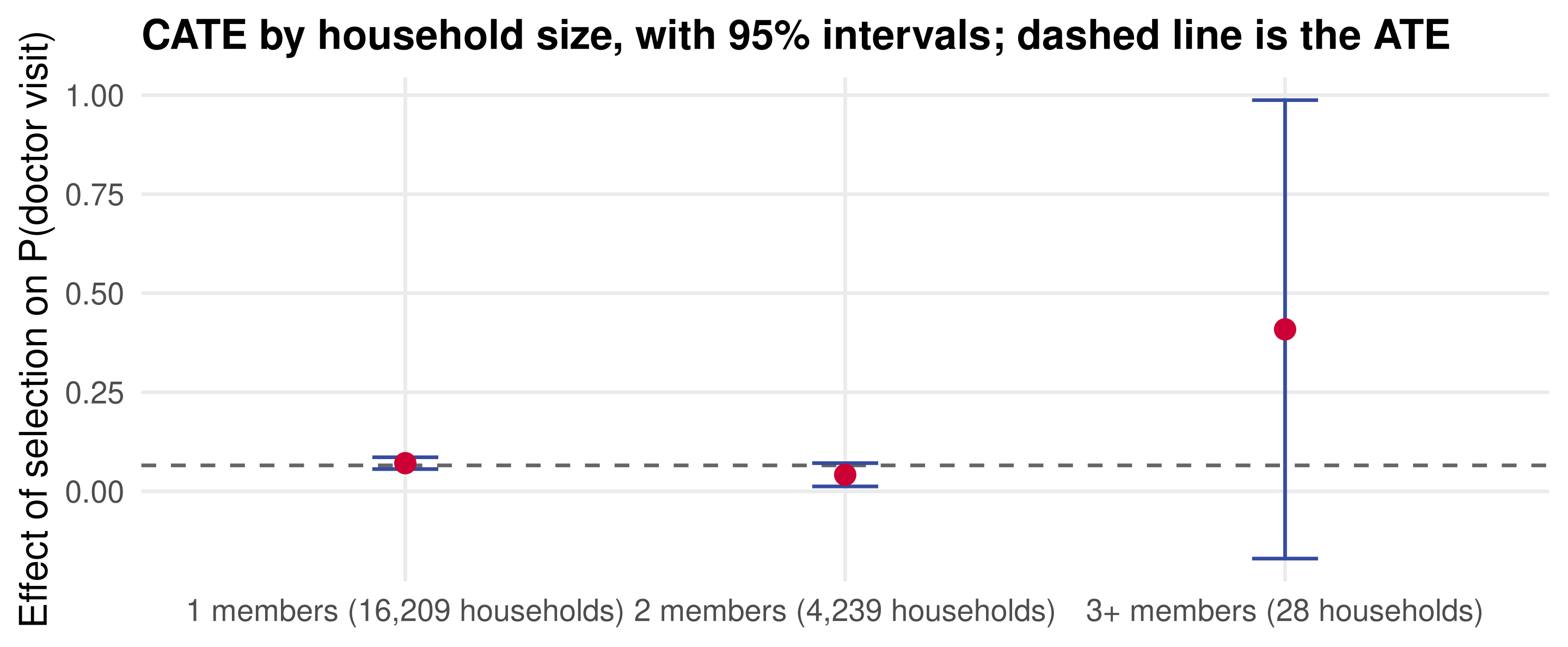
• The CATE is similar for one- and two-person households and imprecisely large for three or more, where there are only 28 households.
• With a constant CATE the model is Y_i = \beta D_i + f(0, X_i) + U_i, so the treatment coefficient in lm(yhh ~ selectedhh + numhh_hh) is the ATE: 0.0653 (s.e. 0.0066), close to the 0.0655 above.

Even with a constant CATE the control must be flexible: household size enters through indicators, not as a number, because f(0, x) need not be linear in x. The constant-CATE regression is what most applied papers run, and the next section runs it on observational data.

Checkpoint: experiments

1. Oregon’s ITT effect is 0.057 and the LATE about 0.19. Which number answers “what if Oregon extends eligibility to everyone”? Which answers “what if Oregon gave everyone insurance”?
2. Why does the household lottery break the simple difference in means, and why does conditioning on household size repair it?
3. The CATE for households of three or more is 0.41. Should Oregon target large households?

Answers: the ITT, because the policy changes eligibility and compliance will be similar; the LATE answers the second only for compliers, and extending insurance to never-takers may have a different effect; larger households were more likely to be selected, so D is correlated with household size, which affects visits, while within a household-size group assignment is a pure lottery; no, the interval runs from about minus 0.2 to 1 on 28 households, which is consistent with the other two groups.

Controlling for covariates

---

Observational data and unconfoundedness

• Usually there is no lottery: we want the effect of a D_i that units chose or that history assigned.
• The standard approach: find controls X_i and regress Y_i on D_i and X_i.
• The causal interpretation uses the assumption we just made for the Oregon households, selection on observables: D_i is independent of \varepsilon_i conditional on X_i. In this setting it is also called unconfoundedness: X_i contains every “confounder” that moves both treatment and outcome.

Warning

In Oregon we knew how D was assigned, so the assumption was a fact about the lottery. With observational data it is a hope about a process we did not design. Everything in this section is about checking that hope and about estimating well when there are many controls.

The language of the treatment effects literature (treatment, controls, propensity score) is used with observational data all the time. The assumption does not become more plausible because the vocabulary is borrowed from experiments.

Abortion and crime

• Roe v. Wade (1973) legalized abortion nationwide; a few states had legalized it shortly before.
• US crime fell sharply in the 1990s.
• Donohue and Levitt (2001): unwanted pregnancies are aborted, children are raised by parents who are ready for them, and eighteen years later there are fewer criminals. The paper was made famous by Freakonomics.

The regressions are at the level of state i and year t (panel data):

• Y_{it}: log murders per capita in state i, year t, de-trended;
• D_{it}: the “effective” abortion rate, abortions eighteen years earlier weighted by the ages of people who commit murder;
• X_{it}: things associated with both unwanted pregnancies and crime: prisoners, police, unemployment, income, poverty, welfare generosity, gun laws, beer.

Does selection on observables with these controls make sense? Put the doubt aside; the regressions are instructive either way.

[Sources] - Donohue and Levitt (2001), QJE 116(2). The data and specification follow Taddy, Business Data Science, chapter 6, which also uses them to introduce the double lasso; Belloni, Chernozhukov and Hansen (2014) use a different specification of the same study.

The data

crime <- read.table("data/abortion.dat", skip = 1, sep = "\t")
names(crime) <- c("state", "year", "pop", "y_viol", "y_prop", "y_murd",
                  "a_murd", "a_viol", "a_prop", "prison", "police",
                  "ur", "inc", "pov", "afdc", "gun", "beer")
crime <- crime[!(crime$state %in% c(2, 9, 12)), ]        # drop Alaska, DC and Hawaii
crime <- crime[crime$year > 84 & crime$year < 98, ]      # complete data for 1985 to 1997
crime$pop <- log(crime$pop)
y <- crime$y_murd                                        # outcome: de-trended log murder rate
d <- crime$a_murd                                        # treatment: effective abortion rate
trend <- crime$year - 85                                 # linear time trend
state <- factor(crime$state)                             # state fixed effects
controls <- crime[, c("pop", "prison", "police", "ur", "inc", "pov", "afdc", "gun", "beer")]
dim(controls)

## [1] 624   9

48 states for 13 years. The controls: log population, log lagged prisoners and police per capita, the unemployment rate, income, the poverty rate, welfare (AFDC) generosity fifteen years earlier, a concealed-weapons law indicator, and beer consumption per capita.

y, d, trend and state are kept as vectors outside the controls data frame so that the formula shorthand “.” below means “all the controls” and “.^2” means “all controls and their pairwise interactions”. The notes name the trend t and the state s; here they are spelled out to avoid shadowing R’s transpose function.

The original specification

A constant CATE, state effects, a linear trend and the controls:

orig <- glm(y ~ d + trend + state + ., data = controls)
round(summary(orig)$coef["d", ], 4)

##   Estimate Std. Error    t value   Pr(>|t|) 
##    -0.2098     0.0411    -5.1059     0.0000

• The effective abortion rate has a negative and highly significant coefficient: more abortions eighteen years ago, fewer murders today. Donohue and Levitt (2001) obtain the same sign with standard errors that allow for heteroskedasticity and serial correlation.

Is it plausible? One popular check from empirical economics: run the same specification with a treatment or an outcome that should have no effect.

We do not adjust the standard errors here; the point is the specification, not the inference. The next three slides are the placebo exercise that undermines it.

Placebo treatments and A/A tests

• In Oregon, the departure from pure randomization was visible and easy to fix. Here nothing is visible. What can we check?
• Rerun the specification with a placebo treatment or outcome: a variable for which a nonzero effect is implausible. In a clinical trial the placebo catches patients reporting improvement with an inert pill; here it catches us finding effects with a bogus specification.

The tech-sector version: A/A tests. Treatment and control are both shown design A, so the measured difference should be zero. A significant difference means the randomization was done badly:

• the same person visits on several devices and sees both A and B;
• users who clear cookies drop out of the measurement (attrition);
• a complex routing tree sends only one type of user to the page being tested, so randomization happened at the wrong level.

The placebo does not prove the specification is wrong; it shows that the specification produces effects where there should be none, which is a reason to distrust the effect where there might be one.

Do cell phones fight crime?

Cell-phone subscriptions per capita, by year, as the placebo treatment:

cell <- read.csv("data/us_cellphone.csv")
cellrate <- 5 * cell$subscribers / (1000 * cell$pop)     # subscribers per person, rescaled
phone <- cellrate[trend + 1]                              # match each state-year to its year
cell_reg <- glm(y ~ phone + trend + state + ., data = controls)
round(summary(cell_reg)$coef["phone", ], 4)

##   Estimate Std. Error    t value   Pr(>|t|) 
##    -0.3721     0.0693    -5.3673     0.0000

• Cell phones “reduce” murder, with a t statistic of -5.4. Faster calls to the police? Perhaps. A more likely explanation is on the next slide.

Subscribers are in persons and population in thousands, so subscribers/(1000 pop) is the share of the population with a subscription; the factor 5 only rescales it to run from 0 to 1 over the sample, like the abortion rate. The scaling does not affect the t statistic.

Both “treatments” are the same curve

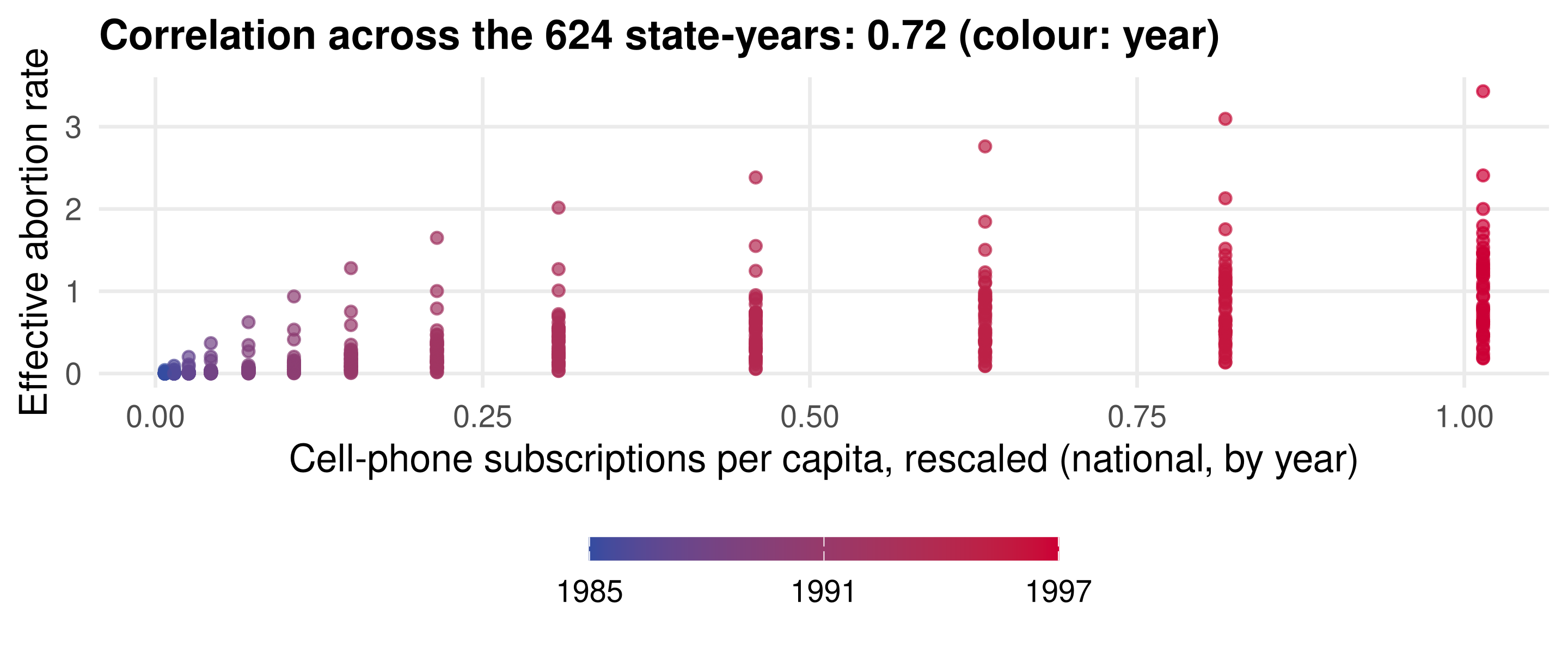
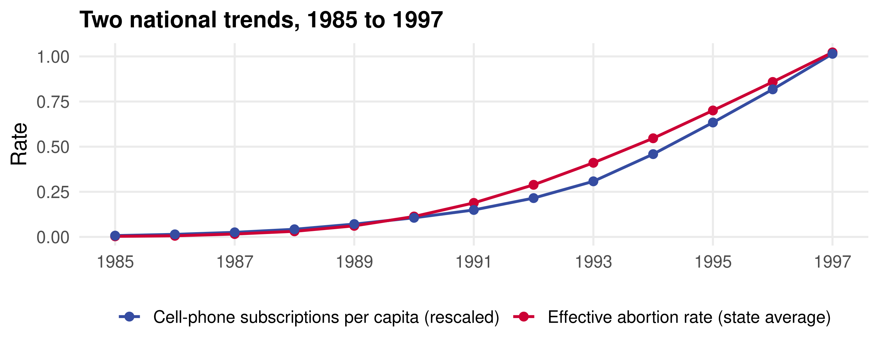
• Both series grew quadratically over 1985 to 1997 (the opening figure). The linear trend absorbs the linear part; the curvature is left for whichever regressor has it, and both do.
• The abortion coefficient may be picking up the same curvature. The fix is to control more flexibly.

The scatter also shows why the two “treatments” are nearly interchangeable in a regression: within a year the abortion rate varies across states, but the dominant variation in both is the common upward curve.

High-dimensional controls

Year indicators instead of a linear trend, state-specific effects of technology adoption, and all squares and interactions of the controls:

trend <- factor(trend)
interact <- glm(y ~ d + trend + phone * state + .^2, data = controls)
round(summary(interact)$coef["d", ], 4)

##   Estimate Std. Error    t value   Pr(>|t|) 
##     0.2797     0.1807     1.5477     0.1224

dim(model.matrix(interact))

## [1] 624 154

• The sign of the abortion coefficient has switched and it is no longer significant.
• 154 regressors for 624 observations. OLS still runs, but with this many controls we may worry about its performance and reach for a regularized estimator.

“.^2” expands to the nine controls plus their 36 pairwise products; “phone * state” adds a state-specific slope on cell-phone adoption. The factor “trend” replaces the straight line with thirteen year effects, so any common curve, quadratic or otherwise, is absorbed.

The lasso on the same specification

set.seed(0)                                               # cross-validation folds
state_all <- factor(state, levels = c(NA, levels(state)), exclude = NULL)   # keep every state
DX <- model.matrix(~ d + trend + phone * state_all + .^2 - 1, data = controls)
cv_lasso <- cv.glmnet(DX, y)
c(lambda.1se = unname(coef(cv_lasso, s = "lambda.1se")["d", ]),
  lambda.min = unname(coef(cv_lasso, s = "lambda.min")["d", ]))

##  lambda.1se  lambda.min 
## -0.10799933 -0.01977922

c(sum(coef(cv_lasso, s = "lambda.1se") != 0), sum(coef(cv_lasso, s = "lambda.min") != 0))

## [1]  59 102

• The point estimate is negative again, smaller than in the original specification, and it changes by a factor of five between the two rules for \lambda.
• Should we trust a lasso coefficient as an estimate of a causal effect?

state_all adds an explicit NA level so that model.matrix() keeps every state when the intercept is dropped with “- 1”, the same device as naref() in the gamlr package. The lasso then gets to shrink each state effect rather than treating one state as the baseline.

Why a lasso coefficient is not an estimate

The lasso was built for prediction. For a single coefficient it has two problems:

• Omitted controls. If D is highly correlated with a control (abortions with cell phones, say), the lasso tends to keep one and drop the other: the penalty punishes the second variable and prediction gains little from it. A dropped control is an omitted variable, and its effect is loaded onto D.
• Instability. Which variables survive depends on the folds and on \lambda, so the treatment coefficient moves around for reasons that have nothing to do with the effect.

The double lasso fixes the first problem by running a second lasso, of D on X, and keeping every control that predicts treatment. A control that predicts D is a potential source of selection bias even if it predicts Y poorly.

The next slide gives the theorem that explains why two regressions are the natural number.

Regularization bias: shrinking the coefficient on a confounder towards zero leaves part of its effect in the treatment coefficient. The second lasso identifies which confounders matter for selection and refuses to let them be shrunk away.

The Frisch–Waugh–Lovell theorem

The OLS coefficient on D in a regression of Y on D and X is numerically identical to the coefficient from:

1. regress D on X and keep the residuals \hat V_i;
2. regress Y_i (or the residuals of Y on X) on \hat V_i.

y_resid <- glm(y ~ trend + phone * state + .^2, data = controls)$residuals
d_resid <- glm(d ~ trend + phone * state + .^2, data = controls)$residuals
c(full = unname(coef(interact)["d"]), residuals = unname(coef(lm(y_resid ~ d_resid))[2]),
  y_on_dresid = unname(coef(lm(y ~ d_resid))[2]))

##        full   residuals y_on_dresid 
##   0.2797107   0.2797107   0.2797107

The double lasso replaces OLS with the lasso in each step. Two regressions, hence “double”; the second step removes the omitted-variable bias of a single lasso, hence “debiased”.

The proof is a projection argument (the residual-maker matrix is idempotent and symmetric); we verify it numerically instead. The treatment coefficient depends on D only through the part of D that X cannot explain, which is exactly where selection on observables says the causal variation lives.

The debiased lasso of Zhang and Zhang

Augment the outcome regression with a treatment regression: Y_i = D_i \beta + X_i'\gamma + U_i, \qquad D_i = X_i'\delta + V_i. For binary D, X_i'\delta is a linear propensity score. Run the lasso on each, keep the residuals \hat U_i and \hat V_i, and correct the lasso coefficient: \hat\beta_{ZZ} = \hat\beta_{\text{lasso}} + \frac{\sum_i \hat V_i \hat U_i}{\sum_i \hat V_i D_i} = \frac{\sum_i \hat V_i\,(Y_i - X_i'\hat\gamma_{\text{lasso}})}{\sum_i \hat V_i D_i}.

• The second form is the FWL second step with \hat V_i as the instrument-like regressor: it is OLS of Y - X'\hat\gamma on D along the residual direction.
• Standard error under homoskedasticity, \mathbf{E}[U_i^2 \mid D_i, X_i] = \sigma^2: \widehat{\operatorname{se}}(\hat\beta_{ZZ}) = \sqrt{\hat\sigma^2 \frac{\sum_i \hat V_i^2}{\bigl(\sum_i \hat V_i D_i\bigr)^2}}, \qquad \hat\sigma^2 = \frac{1}{n}\sum_i \hat U_i^2.

[Sources] - Zhang and Zhang (2014), JRSS-B; the same idea appears in van de Geer, Bühlmann, Ritov and Dezeure (2014) and Javanmard and Montanari (2014). The theory uses a fixed lambda of order sqrt(log(d)/n); we use cross-validation, which the theory does not quite cover.

The debiased lasso in R

beta_lasso <- coef(cv_lasso, s = "lambda.1se")["d", ]
u_hat <- y - predict(cv_lasso, DX, s = "lambda.1se")                # outcome residuals
Xcontrols <- model.matrix(~ trend + phone * state_all + .^2 - 1, data = controls)
cv_d_on_x <- cv.glmnet(Xcontrols, d)                                # the treatment regression
v_hat <- d - predict(cv_d_on_x, Xcontrols, s = "lambda.1se")        # treatment residuals
beta_zz <- beta_lasso + sum(v_hat * u_hat) / sum(v_hat * d)
se_zz <- sqrt(mean(u_hat^2) * sum(v_hat^2) / sum(v_hat * d)^2)
round(c(lasso = beta_lasso, debiased = beta_zz, se = se_zz), 4)

##    lasso debiased       se 
##  -0.1080  -0.0864   0.0513

• The debiased estimate is smaller in magnitude than the lasso’s and still negative, with a standard error a third of the OLS one. Hold that thought: two slides on, we ask whether the small standard error should be believed.

The treatment lasso keeps 71 controls at lambda.1se with these folds. The correction term is the covariance of the two residuals scaled by the covariance of the treatment residual with D; when the lasso has shrunk a confounder, the residuals are correlated and the correction is large.

Post-double-selection

Belloni, Chernozhukov and Hansen (2014) use the two lassos to select, then run OLS:

1. lasso of D on X (done: cv_d_on_x);
2. lasso of Y on X, without D;
3. OLS of Y on D and the union of the controls selected in steps 1 and 2.

cv_y_on_x <- cv.glmnet(Xcontrols, y)
keep <- union(which(coef(cv_y_on_x, s = "lambda.1se") != 0),
              which(coef(cv_d_on_x, s = "lambda.1se") != 0))      # indices count the intercept first
length(keep)

## [1] 110

X1 <- cbind(1, Xcontrols)
pds <- lm(y ~ d + X1[, keep] - 1)
round(coef(summary(pds))["d", ], 4)

##   Estimate Std. Error    t value   Pr(>|t|) 
##     0.2355     0.1470     1.6017     0.1098

• Most of the controls come back and the estimate returns to the OLS value of the full specification, with a smaller standard error. The two double lassos disagree in sign; before choosing, ask how stable each is.

Post-selection OLS removes the shrinkage of the lasso coefficients; the union protects against dropping a confounder that predicts only one of Y and D. Here the selection keeps 110 of 155 columns, so the OLS is nearly the full regression and the estimate is nearly its coefficient.

How stable are these numbers?

The only randomness is the assignment of folds in cv.glmnet(). Repeat everything with ten seeds:

double_lasso <- function(seed) {
  set.seed(seed)
  cv_yd <- cv.glmnet(DX, y); cv_dx <- cv.glmnet(Xcontrols, d); cv_yx <- cv.glmnet(Xcontrols, y)
  u <- y - predict(cv_yd, DX, s = "lambda.1se"); v <- d - predict(cv_dx, Xcontrols, s = "lambda.1se")
  keep <- union(which(coef(cv_yx, s = "lambda.1se") != 0), which(coef(cv_dx, s = "lambda.1se") != 0))
  c(lasso = coef(cv_yd, s = "lambda.1se")["d", ],
    debiased = coef(cv_yd, s = "lambda.1se")["d", ] + sum(v * u) / sum(v * d),
    n_kept = length(keep), pds = unname(coef(lm(y ~ d + X1[, keep] - 1))["d"]))
}
stability <- t(sapply(0:9, double_lasso)); rownames(stability) <- paste("seed", 0:9)
round(stability, 3)

##         lasso debiased n_kept    pds
## seed 0 -0.108   -0.086    110  0.236
## seed 1 -0.118    0.000    116  0.201
## seed 2 -0.118    0.048    117  0.186
## seed 3 -0.113    0.045    117  0.186
## seed 4 -0.121   -0.038    112  0.161
## seed 5 -0.121   -0.029    113  0.174
## seed 6 -0.118   -0.011    115  0.205
## seed 7 -0.130   -0.076    107  0.278
## seed 8 -0.130   -0.141     69 -0.078
## seed 9 -0.118    0.072    118  0.209

Seed 0 reproduces the slides above. The lasso coefficient itself barely moves; the debiased estimate changes sign across seeds and the post-double-selection estimate ranges widely, with one seed selecting far fewer controls and flipping sign. The spread across seeds is of the same order as the reported standard errors.

When to use the double lasso

• The theory was built for d \gg n. When n > d and OLS with all the controls is valid, the double lasso is asymptotically equivalent to that OLS: it cannot do better.
• So if we can run OLS and the double lasso reports a much smaller standard error, be suspicious. Here the fold-to-fold spread of the estimates is as large as the standard errors claim to be, which is the same warning.
• This is the opposite of the prediction case, where the lasso beats OLS even when n > d as long as the true coefficients are small.
• When d > n, OLS is impossible and the double lasso is a good way to get a coefficient and a standard error.

Cross-fitting (“double machine learning”). Compute \hat V_i and \hat U_i for fold k from models fitted on the other folds. Not needed for the lasso, but it lets forests or neural networks play the role of the two regressions without their overfitting biasing \hat\beta (Chernozhukov et al. 2018).

[Sources] - Wüthrich and Zhu (2021), REStat, on the finite-sample omitted-variable bias of lasso-based inference and Monte Carlo evidence; Taddy, Business Data Science, chapter 6, on cross-fitting (p. 177 of the notes’ reference).

Checkpoint: controls

1. The abortion coefficient was significant with a linear trend and insignificant with year effects. Which specification does the cell-phone placebo argue for, and why?
2. Why does the lasso of Y on (D, X) alone risk omitted-variable bias even when the true confounder is in X?
3. In Oregon we had one control with three values; here we have 155. Why does the Frisch–Waugh–Lovell theorem make the number of controls the crux of the problem?

Answers: the placebo “effect” appears only with the linear trend, so a specification that absorbs the common curvature is needed before anything about abortion can be read; the lasso can set the confounder’s coefficient to zero or shrink it when D predicts Y nearly as well, leaving the confounder’s effect in the treatment coefficient; the coefficient on D depends only on the part of D not explained by X, so the quality of the regression of D on X, which gets harder as the number of controls grows, determines the estimate.

Heterogeneous effects with trees and forests

---

From the average effect to who benefits

• So far the target was one number, the ATE, or a few CATEs by hand (household size).
• Often the useful object is a prediction of the treatment effect for a new unit from its covariates: \widehat{\text{CATE}}(X_{n+1}) rather than \hat Y_{n+1}. It decides whom to treat.
  • a scholarship programme: which students gain most from it;
  • personalized medicine: which treatment for which patient, with genetic covariates;
  • marketing: which users get website A after an A/B test.

• The idea: transform the outcome with the propensity score so that the transformed variable has conditional mean \text{CATE}(x). Then run any supervised learner on it: lasso, tree, forest.
• Proposed for trees and forests as “causal trees” and “causal forests” (Athey and Imbens 2016; Wager and Athey 2018). The transformation is more general than the trees.

The prediction target changes, not the toolkit. Everything from lectures 12 to 13 about cross-validation, pruning and bagging applies once we have a variable whose conditional mean is the thing we want.

The transformed outcome

Keep Y_i = g(D_i, X_i, \varepsilon_i), selection on observables, the propensity score p(x) = P(D_i = 1 \mid X_i = x), and write \tau_i = g(1, X_i, \varepsilon_i) - g(0, X_i, \varepsilon_i) for the unit-level effect, so \text{CATE}(x) = \mathbf{E}[\tau_i \mid X_i = x]. Define \tilde Y_i = \frac{Y_i D_i}{p(X_i)} - \frac{Y_i (1 - D_i)}{1 - p(X_i)}.

Claim. \mathbf{E}[\tilde Y_i \mid X_i = x] = \text{CATE}(x). For the first term, Y_i D_i = g(1, x, \varepsilon_i) D_i when X_i = x, and D_i is independent of \varepsilon_i given X_i, so \mathbf{E}\!\left[\frac{Y_i D_i}{p(X_i)} \,\Big|\, X_i = x\right] = \frac{\mathbf{E}[g(1, x, \varepsilon_i) \mid X_i = x]\; P(D_i = 1 \mid X_i = x)}{p(x)} = \mathbf{E}[g(1, x, \varepsilon_i) \mid X_i = x]. The second term gives \mathbf{E}[g(0, x, \varepsilon_i) \mid X_i = x] the same way; the difference is the CATE.

Regress \tilde Y_i on X_i with any method. The fitted function estimates \text{CATE}(x) directly.

Each term reweights the units that received a given treatment by the inverse of the probability of receiving it, so that the reweighted treated units look like the whole population at x. The full derivation with every conditioning step is in the appendix.

Why not regress Y on (D, X) and difference?

We could fit \hat f(d, x) and report \hat f(1, x) - \hat f(0, x), as in Oregon. What is the difference?

• The bias-variance trade-off that sets the lasso penalty, the tree depth and the split points is tuned for the object being fitted. Fitting f(d, x) tunes for the outcome; fitting \tilde Y tunes for the effect.
• Suppose f(1, x) and f(0, x) both vary a lot with x but their difference does not: outcomes depend on x, effects do not. A tree for f needs many leaves; a tree for the CATE needs few. Differencing two big trees gives a noisy difference.

Cost. The regression of \tilde Y on X leaves D out of the predictors, so its error term has more variance; with a weak signal, the estimates are noisy.

Two practical cautions.

• With observational data, p(x) must be estimated and its bias propagates into \tilde Y. Fine when X is low-dimensional and the model is flexible (Hirano, Imbens and Ridder 2003); dangerous otherwise. Today p is known: the data are experimental.
• Treatment assigned at an aggregate level (villages, schools) must be resampled at that level in cross-validation and bagging, or the folds cheat by predicting a household from its neighbours (Athey and Wager 2019, section 1.2).

Causal trees in Athey and Imbens (2016) refine this: they change the splitting criterion to target the effect directly and use honest estimation (section 6) within each leaf. The transformed outcome is the simplest member of the family.

The National Supported Work demonstration

A 1970s job-training programme, randomized among disadvantaged workers; the Dehejia and Wahba (1999) subsample of 185 treated and 260 controls:

nsw <- read.csv("data/dw_experimental_data.csv")
dim(nsw)

## [1] 445  11

Variable	Meaning
re78	Earnings in 1978, after the programme, in thousands of dollars: the outcome
treated	Assigned to the programme
re74, re75	Earnings in 1974 and 1975, before the programme
ue74, ue75	Unemployed (zero earnings) in 1974 and 1975
age, education, black, hispanic, married	Demographics; education in years

[Sources] - LaLonde (1986), AER, first used these data to show that observational methods failed to recover the experimental answer; Dehejia and Wahba (1999), JASA, built this subsample with the 1974 earnings. 185 treated, 260 controls; 31% of the sample had zero earnings in 1978.

Was treatment random?

Assignment was by lottery, so p(x) = p for every x. A logit of treatment on the covariates should find nothing:

glm_treat <- glm(treated ~ . - re78, data = nsw, family = "binomial")
round(coef(summary(glm_treat)), 3)

##              Estimate Std. Error z value Pr(>|z|)
## (Intercept)    -0.474      0.824  -0.575    0.566
## age             0.014      0.014   1.004    0.316
## education       0.050      0.056   0.886    0.376
## blackTRUE      -0.348      0.361  -0.964    0.335
## hispanicTRUE   -0.928      0.507  -1.833    0.067
## marriedTRUE     0.176      0.275   0.640    0.522
## re74           -0.034      0.029  -1.160    0.246
## re75            0.012      0.047   0.259    0.796
## ue74TRUE       -0.152      0.372  -0.408    0.683
## ue75TRUE       -0.372      0.318  -1.171    0.242

No coefficient is significant at 5% and the likelihood-ratio test of all nine has p = 0.23. The description of the programme fits the data.

This is a balance check, the experimental analogue of the placebo test: with a real lottery, the covariates cannot predict treatment. The Hispanic indicator is the closest to significance at p = 0.07, as one of nine tests might be.

The transformed outcome in R

With a constant propensity score, estimate p by the treated share:

p_hat <- mean(nsw$treated)
y_tilde <- nsw$re78 * nsw$treated / p_hat - nsw$re78 * (1 - nsw$treated) / (1 - p_hat)
c(p_hat = p_hat, ATE = mean(y_tilde), diff_in_means = unname(diff(tapply(nsw$re78, nsw$treated, mean))))

##         p_hat           ATE diff_in_means 
##     0.4157303     1.7943424     1.7943424

c(sd_re78 = sd(nsw$re78), sd_y_tilde = sd(y_tilde))

##    sd_re78 sd_y_tilde 
##   6.631492  18.147909

• The mean of \tilde Y is the ATE estimate: the programme raised 1978 earnings by about $1,794 on average. With p(x) = p it equals the difference in means exactly.
• The transformed outcome is almost three times as spread out as earnings. That is the variance cost of leaving D out.

With p constant, mean(y_tilde) = mean(Y | D = 1) − mean(Y | D = 0) algebraically, since the sums of D/p and (1 − D)/(1 − p) over the sample are both n. The standard error of the difference in means is about 0.63, so the ATE is significant at the 1% level.

A linear CATE

lm_cate <- lm(y_tilde ~ . - treated - re78, data = nsw)
round(coef(summary(lm_cate)), 3)

##              Estimate Std. Error t value Pr(>|t|)
## (Intercept)   -14.296      7.211  -1.983    0.048
## age             0.100      0.124   0.802    0.423
## education       1.084      0.488   2.223    0.027
## blackTRUE      -0.186      3.198  -0.058    0.954
## hispanicTRUE   -3.381      4.278  -0.790    0.430
## marriedTRUE     2.729      2.422   1.127    0.261
## re74            0.115      0.239   0.482    0.630
## re75            0.061      0.410   0.149    0.881
## ue74TRUE        8.823      3.261   2.706    0.007
## ue75TRUE       -6.614      2.810  -2.354    0.019

• Little evidence of heterogeneity: education is marginally significant (about $1,100 more per year of schooling), and the two unemployment indicators offset each other. Everything else is noise.

Each coefficient is the change in the CATE per unit of the covariate, since the regression function of y_tilde is the CATE. The R squared of this regression (not shown) is under 4%.

A tree for the CATE

Grow a large tree and prune by cross-validation, as in lecture 13. The unemployment indicators are left out: a tree can find them itself by splitting earnings just above zero.

tree_cate <- tree(y_tilde ~ . - treated - re78 - ue74 - ue75, data = nsw, mindev = 0, mincut = 10)
set.seed(0)
cv_cate <- cv.tree(tree_cate)
(best_size <- cv_cate$size[which.min(cv_cate$dev)])

## [1] 2

prune.tree(tree_cate, best = best_size)

## node), split, n, deviance, yval
##       * denotes terminal node
## 
## 1) root 445 146200  1.794  
##   2) education < 12.5 423 122900  1.005 *
##   3) education > 12.5 22  18000 16.960 *

• The tree finds one split: an estimated effect of about $1,000 for people with twelve or fewer years of schooling and $17,000 for the 22 with more. Nothing else.

With other seeds cv.tree() sometimes chooses the root (one leaf); the ten-fold honest check cv_prune() from lecture 13 also chooses two leaves. The 22 people with more than twelve years of schooling are few, and 15 of them were treated; section 6 asks whether this split survives a fresh sample.

A forest for the CATE

set.seed(0)
rf_cate <- ranger(y_tilde ~ . - treated - re78 - ue74 - ue75, data = nsw, num.trees = 200,
                  min.node.size = 5, importance = "impurity", keep.inbag = TRUE)

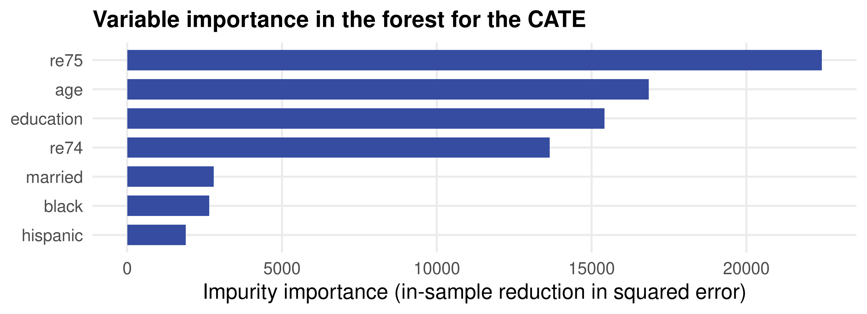
• Harder to read than the tree or the regression. The binary indicators rank low, but each can only be split once, so importance says little about them. keep.inbag = TRUE saves what each tree saw, for the standard errors later.

Impurity importance is computed in sample, so it rewards continuous variables that offer many split points (lecture 13). The forest is 200 trees of minimum node size 5, as in the notes.

What the forest predicts

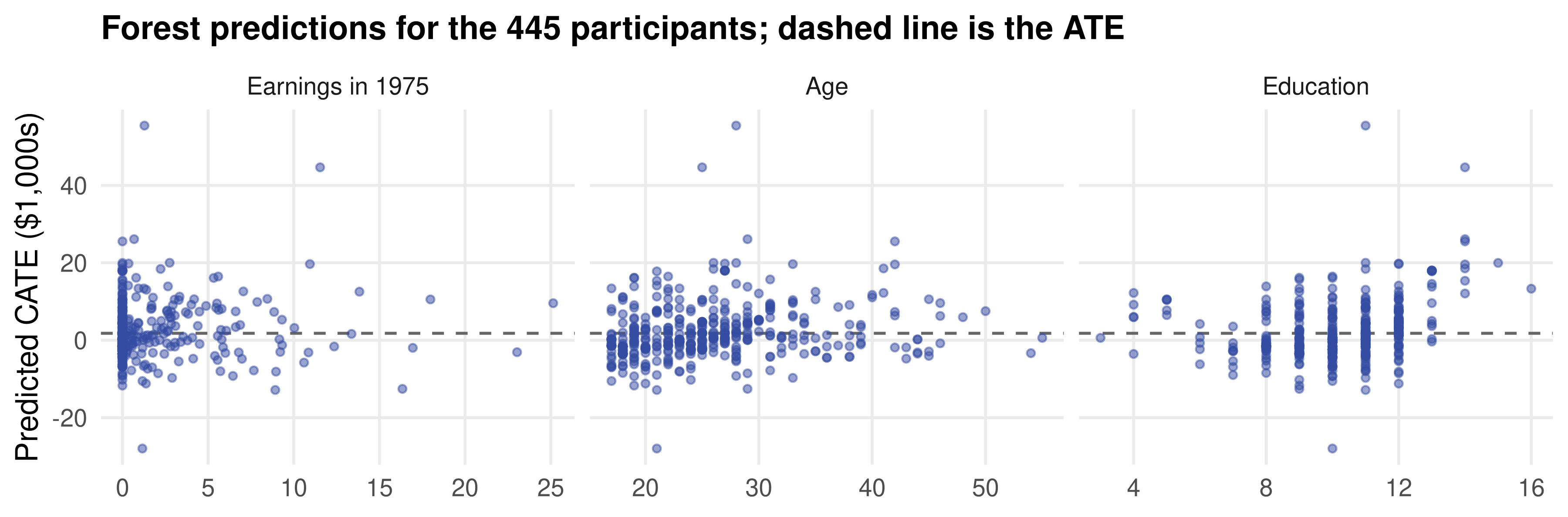
• The predicted effects range from -28 to 55 thousand dollars, around an average effect of 1.8. 8% of participants get a predicted effect below minus $5,000.
• It is implausible that a training programme costs some participants $10,000 a year and earns others $20,000. The forest is probably overfitting.

These are in-sample predictions (each tree votes on observations it was trained on, for the bagged ones), which is what the notes plot. The out-of-bag predictions have a narrower range, from about minus 10 to 27, and the same lack of pattern.

Is there any heterogeneity at all?

A forest is hard to read, but its out-of-bag R^2 answers one question: does X predict the transformed outcome at all?

rf_cate$r.squared

## [1] -0.07023661

• A large R^2 would mean the CATE varies a lot relative to the total variation in \tilde Y. Here it is negative: out of bag, the forest predicts worse than the sample mean of \tilde Y, the constant ATE.
• Two conclusions: there is little evidence that \text{CATE}(x) varies, and the forest overfits.

Now the confidence intervals. ranger computes a standard error for each prediction by the infinitesimal jackknife of Wager, Hastie and Efron (2014):

lower <- rf_pred$predictions - 2 * rf_pred$se
upper <- rf_pred$predictions + 2 * rf_pred$se
c(lower_above_ATE = mean(lower > mean(y_tilde)), upper_below_ATE = mean(upper < mean(y_tilde)), upper_below_0 = mean(upper < 0))

## lower_above_ATE upper_below_ATE   upper_below_0 
##       0.1415730       0.3033708       0.1370787

The intervals say the CATE is “significantly” above or below the average for 44% of participants, and significantly negative for 14%. That contradicts the R^2. Section 6 explains which to believe.

The infinitesimal jackknife uses the in-bag counts saved by keep.inbag to estimate the sampling variance of each bagged prediction. The forest and its intervals are built from the same observations, which is the problem the next section names.

Checkpoint: heterogeneous effects

1. Why does \mathbf{E}[\tilde Y_i \mid X_i = x] equal the CATE only under selection on observables? Where is the assumption used?
2. In the NSW data the forest’s in-sample predictions range over $80,000. Name two reasons the out-of-bag R^2 is the better guide.
3. A marketing team estimates a CATE forest on an A/B test and treats the 20% of users with the highest predicted effect. What could go wrong?

Answers: in factoring E[g(1, x, eps) D | X = x] into E[g(1, x, eps) | X = x] times P(D = 1 | X = x), which needs D independent of eps given X; in-sample predictions reuse the observations that grew the trees, so they fit noise, while out of bag each observation is predicted by trees that never saw it, and the negative value says the structure found in sample does not generalize; the ranking is estimated with the same noise as the predictions, so the top 20% are partly the users with the luckiest noise, and the realized effect in that group will be smaller than predicted (the winner’s curse of section 6).

Honest trees and post-selection inference

---

A confidence interval for a leaf

A tree predicts \hat f(x) by the mean of Y_i over the leaf R_\ell that contains x: \hat f(x) = \bar Y_\ell = \frac{1}{N_\ell}\sum_{i: X_i \in R_\ell} Y_i, \qquad N_\ell = \#\{i : X_i \in R_\ell\}.

The naive interval treats the leaf as a sample: \operatorname{se}(x) = \frac{\widehat{\operatorname{sd}}_\ell}{\sqrt{N_\ell}}, \qquad \widehat{\operatorname{sd}}_\ell^2 = \frac{1}{N_\ell}\sum_{i: X_i \in R_\ell}(Y_i - \bar Y_\ell)^2, \qquad \hat f(x) \pm 2\operatorname{se}(x).

Two things are wrong with it:

1. Selection. The leaf boundaries were chosen by looking at the same Y_i: the tree grouped observations because their Y values were similar. The interval ignores that.
2. Bias. The leaf mean averages over X_i \neq x; if f varies inside the leaf, \bar Y_\ell is biased for f(x).

Honest trees fix (1) by sample splitting. For (2) we either reinterpret the interval as one for the leaf average, or undersmooth the tree, as for nonparametric regression intervals.

Problem (1) is the one that makes intervals too narrow after any data-driven model choice; problem (2) is the usual bias of local averaging. Both appear in the forest intervals of section 5.

Honest trees

A simple version of the algorithm of Athey and Imbens (2016):

1. Split the sample into two folds. Grow and prune a tree on fold 1 only.
2. Estimate on fold 2. For each leaf R_\ell of that tree, use only the fold-2 observations in it: \hat f(x) = \bar Y_{2,\ell} = \frac{1}{N_{2,\ell}}\sum_{i \in \text{fold 2}:\, X_i \in R_\ell} Y_i, \qquad \operatorname{se}(x) = \frac{\widehat{\operatorname{sd}}_{2,\ell}}{\sqrt{N_{2,\ell}}}, with N_{2,\ell} the number of fold-2 observations in the leaf and \widehat{\operatorname{sd}}_{2,\ell}^2 = \frac{1}{N_{2,\ell}}\sum_{i \in \text{fold 2}:\, X_i \in R_\ell}(Y_i - \bar Y_{2,\ell})^2.

The leaf boundaries are fixed before fold 2 is looked at, so within a leaf the fold-2 observations are an ordinary sample and the ordinary interval applies.

The price is data: half the sample picks the model, half estimates it. The next slides show what it buys.

The notes’ statement of the fold-2 standard deviation is incomplete; the formula above is the intended one (the code uses the sample standard deviation with N − 1, which makes no difference at these leaf sizes).

A simulation with nothing to find

One covariate, a constant regression function \mathbf{E}[Y \mid X] = 0, and a tree grown until leaves have twenty observations, with no pruning:

set.seed(0)
n <- 1000; x <- runif(n); y <- rnorm(n)
simple_tree <- tree(y ~ x, mindev = 0, mincut = 20)

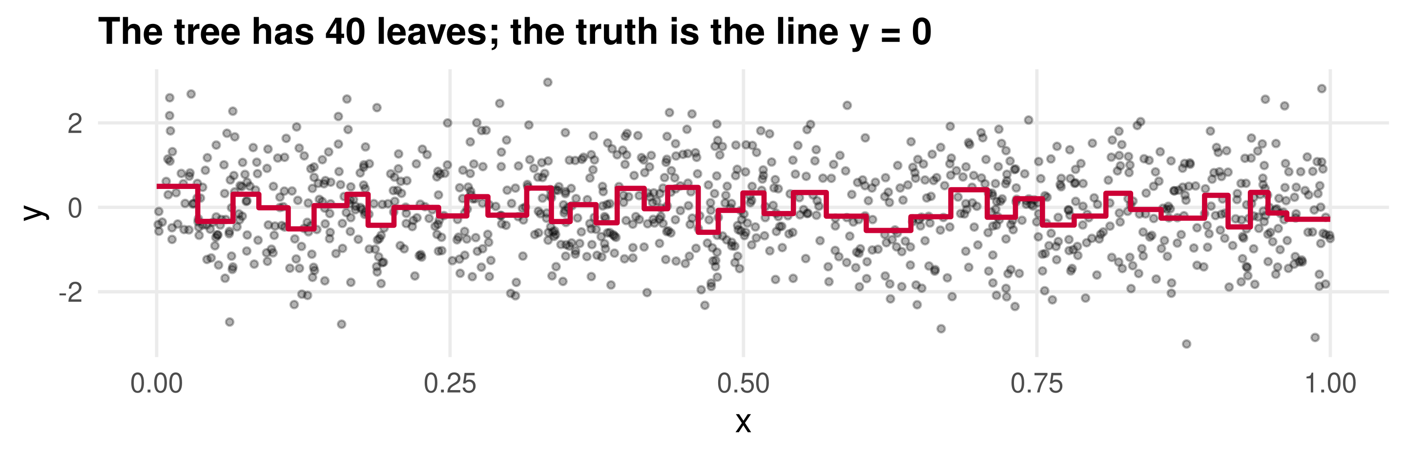
The fit wiggles although there is nothing to fit. We would like each leaf’s interval to contain the truth, 0, about 95% of the time.

mindev = 0 forces the tree to keep splitting; mincut = 20 keeps at least twenty observations in each leaf so that an interval can be formed. The same tree would be a reasonable first stage before pruning.

Naive coverage

The naive interval for each observation’s leaf, and the share that contain the true value 0:

leaves <- predict(simple_tree, type = "where")             # the leaf of each observation
naive <- tibble(y, leaf = leaves) |> group_by(leaf) |>
  mutate(estimate = mean(y), se = sd(y) / sqrt(n())) |> ungroup()
mean(naive$estimate - 2 * naive$se < 0 & naive$estimate + 2 * naive$se > 0)

## [1] 0.664

• Two thirds, not 95%. The intervals are too narrow because they are centred in the wrong place.
• Why. Suppose a few neighbouring observations happen to have Y_i > 0. The tree finds them and makes them a leaf. The leaf mean is then positive by construction, and the naive standard error, computed within the leaf, does not know that the cut points were chosen to make it so.

This is the winner’s curse of model selection: the leaves are selected for extreme means, so their means are biased away from zero, and the within-leaf standard deviation is biased downwards because similar values were grouped on purpose.

Honest coverage

Grow the tree on a random half, estimate on the other half:

fold1 <- sample(n, size = n / 2)
honest_tree <- tree(y ~ x, mindev = 0, mincut = 20, subset = fold1)
fold2 <- tibble(x = x[-fold1], y = y[-fold1])
fold2$leaf <- predict(honest_tree, newdata = fold2, type = "where")   # fold-2 observations in fold-1 leaves
honest <- fold2 |> group_by(leaf) |> mutate(estimate = mean(y), se = sd(y) / sqrt(n())) |> ungroup()
mean(honest$estimate - 2 * honest$se < 0 & honest$estimate + 2 * honest$se > 0)

## [1] 0.956

• Coverage is restored. The fold-1 tree still has leaves chosen for their extreme fold-1 means, but the fold-2 observations in those leaves are fresh noise with mean zero.
• One data set is one draw. Over 200 simulated data sets (appendix) the naive interval covers about 75% of the time and the honest one about 95%.

The honest tree has about half the leaves (21 against 40) because it is grown on half the data. That is the loss from splitting, and the next slide shows how forests recover it.

Post-selection inference in general

Honest trees are one instance of a general recipe for inference after model selection:

1. Fold 1 selects the model. Trees: grow and prune with cross-validation. Lasso: run cv.glmnet() and record which coefficients are nonzero.
2. Fold 2 estimates it. Trees: leaf means and standard errors from fold 2. Lasso: OLS of Y on the selected covariates in fold 2, with the usual standard errors.

• Honest forests. Splitting wastes half the data for one tree, but swapping the folds gives a second tree, and many random splits give a forest of honest trees. Each tree’s leaves never see the observations that estimate them, which is what the forest intervals of section 5 lacked. Formulas and software are in Wager and Athey (2018) and the grf package.
• Refinements that avoid splitting, by conditioning on the selection event, are in Lee, Sun, Sun and Taylor (2016); a version for heterogeneous effects in experiments is Chernozhukov, Demirer, Duflo and Fernández-Val (2019).

The in-sample forest intervals of section 5 used the infinitesimal jackknife on trees grown on the same observations; the honest forest grows each tree on one subsample and fills its leaves from another, so the same jackknife becomes valid.

What an honest interval estimates

The fold-1 model is random, so the honest interval is for a random target. Take the CATE tree of section 5, one split on education:

## node), split, n, deviance, yval
##       * denotes terminal node
## 
## 1) root 445 146200  1.794  
##   2) education < 12.5 423 122900  1.005 *
##   3) education > 12.5 22  18000 16.960 *

• Had this tree come from fold 1, the fold-2 intervals would be for the average treatment effect within each leaf: for people with at most twelve years of schooling and for people with more. Not for the CATE at every combination of age, race and earnings.
• Another sample would select other leaves, and the intervals would be for other averages. Think of fold 1 as finding the interesting dimensions of heterogeneity and fold 2 as measuring the effect along them.

Warning

If the controls are needed for identification (observational data, estimated propensity scores), a tree that splits only on education controls for nothing else. The same caution applies to post-selection OLS after the lasso, which is why the double lasso puts controls back.

“Honest” refers to the standard errors, not to the target. The interval is valid for whatever leaf average fold 1 happened to define. In an experiment this is fine because every leaf average is a causal quantity; in observational data it is not, unless every confounder is still conditioned on.

Honest CATEs in the NSW data

Fold 1, a random half, grows the tree with the default stopping rules:

set.seed(0)
fold1 <- sample(nrow(nsw), size = round(nrow(nsw) / 2))
tree_fold1 <- tree(y_tilde ~ . - treated - re78 - ue74 - ue75, data = nsw, subset = fold1)
tree_fold1

## node), split, n, deviance, yval
##       * denotes terminal node
## 
##  1) root 222 84090  2.8720  
##    2) education < 12.5 213 71480  1.8890  
##      4) education < 10.5 117 22740 -0.6436 *
##      5) education > 10.5 96 47080  4.9770  
##       10) age < 25.5 57  8129  1.7200 *
##       11) age > 25.5 39 37460  9.7370  
##         22) re74 < 2.17518 30 33240 13.8600  
##           44) re75 < 1.04371 23 12190  8.6020 *
##           45) re75 > 1.04371 7 18330 31.1400 *
##         23) re74 > 2.17518 9  2009 -4.0120 *
##    3) education > 12.5 9  7536 26.1300 *

Six leaves: education first, then age, then 1974 and 1975 earnings. The leaf means run from minus 4 to 31 thousand dollars, which is the fold-1 analogue of the wild forest predictions of section 5. Fold 2 tells us how much of that survives.

Fold 2 estimates the leaves

nsw_fold2 <- nsw[-fold1, ]
nsw_fold2$y_tilde <- y_tilde[-fold1]
nsw_fold2$leaf <- predict(tree_fold1, newdata = nsw_fold2, type = "where")
honest_nsw <- nsw_fold2 |> group_by(leaf) |>
  summarise(label = rownames(tree_fold1$frame)[first(leaf)], estimate = mean(y_tilde),
            se = sd(y_tilde) / sqrt(n()), n = n()) |>
  mutate(fold1_estimate = tree_fold1$frame$yval[leaf])
honest_nsw |> select(label, fold1_estimate, estimate, se, n) |>
  mutate(across(c(fold1_estimate, estimate, se), ~ round(.x, 2))) |> as.data.frame()

##   label fold1_estimate estimate   se   n
## 1     4          -0.64    -0.33 1.43 117
## 2    10           1.72     1.09 2.15  49
## 3    44           8.60    -0.99 3.17  29
## 4    45          31.14     8.10 7.01   5
## 5    23          -4.01    -0.35 5.61  10
## 6     3          26.13    10.62 7.67  13

• label is the node number in the tree printout; fold1_estimate is the leaf mean fold 1 reported, and estimate what fold 2 finds in the same leaf.
• The two leaves with large fold-1 effects (nodes 45 and 3, $31,000 and $26,000) shrink to $8,000 and $11,000 with standard errors of the same size.

The notes compute these estimates with predict(tree, data = …, type = “where”); predict.tree() takes newdata, not data, so that call returns the fold-1 leaves of the fold-1 observations and the fold-2 outcomes are matched to the wrong rows (the printed leaf sizes equal the fold-1 ones). The code here passes newdata; the estimates and standard errors differ from the notes’ printout, and the conclusion is the same.

Fold 1 against fold 2

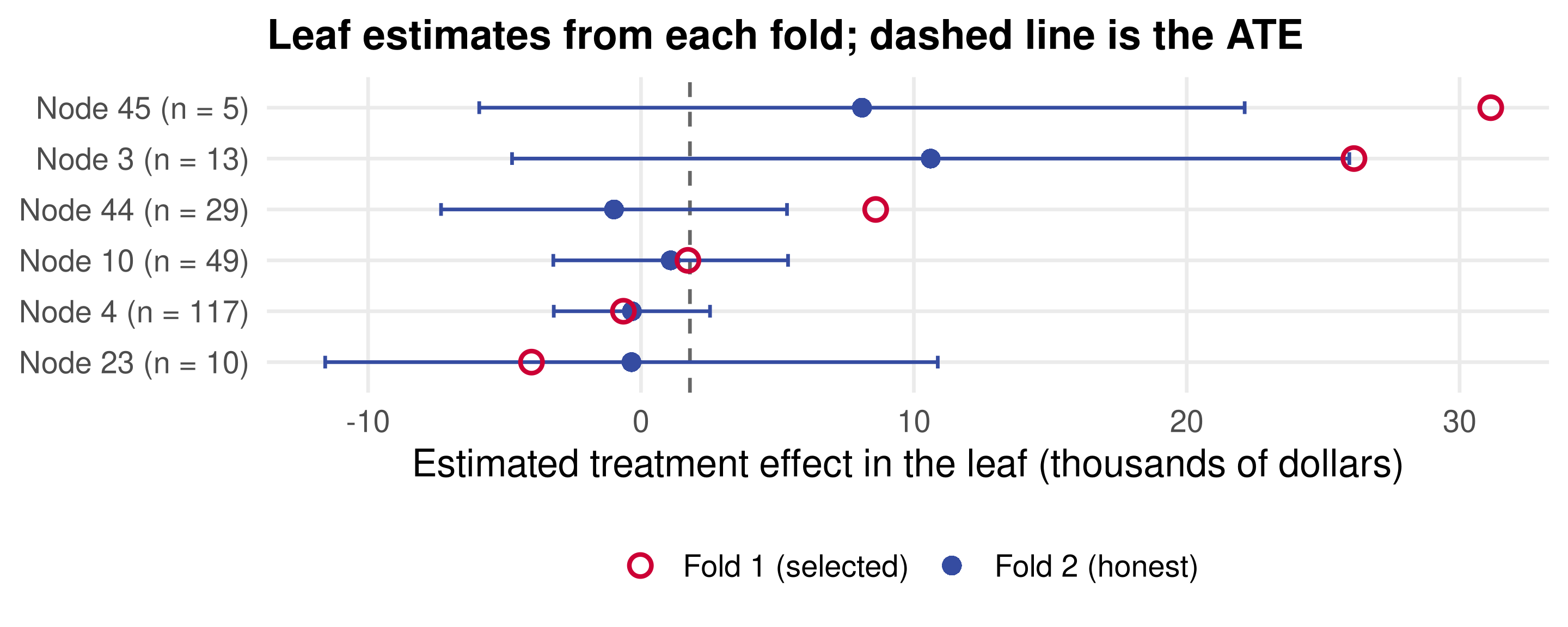
• Every honest interval contains the ATE, so the shares of participants whose interval lies above or below it, the numbers that were 14% and 30% for the forest, are both 0%. Little evidence of heterogeneity, in agreement with the out-of-bag R^2.
• There are only six intervals, one per leaf, and some leaves hold five or ten people, for whom the normal approximation is a stretch.

The fold-1 estimates are the winner’s curse in one picture: leaves were chosen because their fold-1 means were extreme, and the fresh fold-2 means regress towards the overall effect. The right reading is a confidence interval for the average effect among, say, people with more than twelve years of education, which is 10.6 plus or minus 15.

Checkpoint: honest inference

1. Why does the honest interval have the right coverage even though the fold-1 tree was chosen to make leaf means extreme?
2. The forest intervals of section 5 found “significant” heterogeneity for nearly half of the participants; the honest intervals found none. Explain the discrepancy in one sentence.
3. After selecting a model with the lasso on fold 1, why run OLS rather than the lasso on fold 2?

Answers: the extremeness is a property of the fold-1 values, and the fold-2 observations in the same leaf are an independent sample whose mean and standard error are the ordinary ones; the forest’s intervals were computed from the same observations that defined its leaves, so they inherit the selection bias that the simulation showed cuts coverage to two thirds; the lasso shrinks coefficients, so its estimates are biased and have no standard errors, while OLS on a model fixed in advance has both.

Causal inference in one page

A causal effect is defined by a counterfactual. Y = g(D, \varepsilon); the unit-level effect g(1, \varepsilon) - g(0, \varepsilon) compares two potential outcomes, one of which is never observed. State the intervention and what it holds fixed.

Regression gives the average effect under one assumption. With D independent of \varepsilon, the difference in means is the ATE. Otherwise \hat\beta carries the selection term \operatorname{Cov}(\varepsilon, D)/\operatorname{Var}(D), which helps prediction and ruins intervention.

Experiments make the assumption true; controls make it conditional. Randomize, and remember what was actually randomized (eligibility, households). Condition on X under selection on observables, flexibly, and read the CATE off \hat f(1, x) - \hat f(0, x). Placebo treatments test the specification.

One lasso is biased for a coefficient; two are not. By Frisch–Waugh–Lovell, the treatment coefficient lives in the part of D that X cannot explain. The double lasso regularizes both regressions and is the tool when d > n; when n > d, trust OLS and be suspicious of a smaller standard error.

ML estimates heterogeneous effects from the transformed outcome, and sample splitting makes the inference honest. \tilde Y has conditional mean \text{CATE}(x); any learner can fit it. Intervals from the same data that chose the model are too narrow; fold 1 selects, fold 2 estimates.

Reading and data sources

• Angrist and Pischke, Mastering ’Metrics (2015), chapters 1 to 3: experiments, regression and instruments, with the Oregon experiment as a running example.
• Taddy, Business Data Science (2019), chapters 5 and 6: the Oregon, abortion and cell-phone analyses, the double lasso and cross-fitting.
• Finkelstein et al. (2012), the Oregon Health Insurance Experiment; Donohue and Levitt (2001), abortion and crime; LaLonde (1986) and Dehejia and Wahba (1999), the NSW data.
• Belloni, Chernozhukov and Hansen (2014), post-double-selection; Zhang and Zhang (2014), the debiased lasso; van de Geer et al. (2014) and Javanmard and Montanari (2014), related; Chernozhukov et al. (2018), double machine learning; Wüthrich and Zhu (2021), when lasso-based inference misleads.
• Athey and Imbens (2016), causal and honest trees; Wager and Athey (2018), causal forests; Athey and Wager (2019), an application; Wager, Hastie and Efron (2014), forest standard errors; Hirano, Imbens and Ridder (2003), estimated propensity scores.
• Lee, Sun, Sun and Taylor (2016), exact post-selection inference; Chernozhukov, Demirer, Duflo and Fernández-Val (2019), generic ML inference on heterogeneous effects.

Additional derivations and code

---

Optional material for reference and practice

OLS on a binary regressor is a difference in means

Let n_1 be the number of treated units, \bar D = n_1/n, and \bar Y = \bar D\, \bar Y_1 + (1 - \bar D)\, \bar Y_0. Then \widehat{\operatorname{Cov}}(Y, D) = \frac{1}{n}\sum_i (D_i - \bar D)\, Y_i = \bar D\, \bar Y_1 - \bar D\, \bar Y = \bar D\,(\bar Y_1 - \bar Y) = \bar D (1 - \bar D)(\bar Y_1 - \bar Y_0), using \bar Y_1 - \bar Y = (1 - \bar D)(\bar Y_1 - \bar Y_0). For a binary variable \widehat{\operatorname{Var}}(D) = \bar D(1 - \bar D), so \hat\beta = \frac{\widehat{\operatorname{Cov}}(Y, D)}{\widehat{\operatorname{Var}}(D)} = \bar Y_1 - \bar Y_0.

• The intercept is \bar Y_0, and the fitted values are the two group means: a regression on a binary D is saturated.
• With a saturated set of controls interacted with D, as in the Oregon household regression, the same holds within each value of X, which is why the interaction coefficients are differences of CATEs.

The transformed outcome, in full

With X_i = x fixed, Y_i D_i = g(1, x, \varepsilon_i)\, D_i because the product is zero unless D_i = 1, in which case Y_i = g(1, x, \varepsilon_i). Hence \mathbf{E}\!\left[\frac{Y_i D_i}{p(X_i)} \,\Big|\, X_i = x\right] = \frac{\mathbf{E}[g(1, x, \varepsilon_i)\, D_i \mid X_i = x]}{p(x)}. Selection on observables says D_i and \varepsilon_i are independent given X_i = x, so the expectation of the product factors: \mathbf{E}[g(1, x, \varepsilon_i)\, D_i \mid X_i = x] = \mathbf{E}[g(1, x, \varepsilon_i) \mid X_i = x]\; \mathbf{E}[D_i \mid X_i = x] = \mathbf{E}[g(1, x, \varepsilon_i) \mid X_i = x]\; p(x). The p(x) cancels. The second term of \tilde Y_i uses 1 - D_i and 1 - p(x) in the same way, so \mathbf{E}[\tilde Y_i \mid X_i = x] = \mathbf{E}[g(1, x, \varepsilon_i) \mid X_i = x] - \mathbf{E}[g(0, x, \varepsilon_i) \mid X_i = x] = \text{CATE}(x).

• The weights 1/p(x) and 1/(1 - p(x)) are the inverse probability weights of Horvitz and Thompson; averaging \tilde Y_i over the sample gives the inverse-probability-weighted ATE estimator.
• With p(x) = p constant, \frac{1}{n}\sum_i \tilde Y_i = \frac{1}{n p}\sum_{i: D_i = 1} Y_i - \frac{1}{n(1 - p)}\sum_{i: D_i = 0} Y_i, which equals \bar Y_1 - \bar Y_0 exactly when p is the treated share.

Coverage over many simulated data sets

The naive and honest coverage on one data set were 0.664 and 0.956. Averaged over 200 data sets:

coverage <- function(y, leaf) {                     # share of observations whose leaf interval contains 0
  est <- tapply(y, leaf, mean)[as.character(leaf)]
  se <- (tapply(y, leaf, sd) / sqrt(table(leaf)))[as.character(leaf)]
  mean(abs(est) < 2 * se)
}
set.seed(1)
mc <- replicate(200, {
  x <- runif(n); y <- rnorm(n)
  full <- tree(y ~ x, mindev = 0, mincut = 20)
  f1 <- sample(n, n / 2)
  half <- tree(y ~ x, mindev = 0, mincut = 20, subset = f1)
  c(naive = coverage(y, predict(full, type = "where")),
    honest = coverage(y[-f1], predict(half, newdata = data.frame(x = x[-f1]), type = "where")))
})
round(rowMeans(mc), 3)

##  naive honest 
##  0.747  0.943

A note on notation

The deck writes Y_i = g(D_i, X_i, \varepsilon_i) and assumes D_i independent of \varepsilon_i given X_i. Two alternatives are common:

• Let u_i = (X_i, \varepsilon_i) and write Y_i = g(D_i, u_i); the assumption becomes “D_i independent of u_i given X_i”, which is the same statement because conditioning on X_i leaves only \varepsilon_i random.
• Potential outcomes notation: Y_i^*(d) = g(d, X_i, \varepsilon_i) and Y_i = Y_i^*(D_i); the assumption is that (Y_i^*(0), Y_i^*(1)) are independent of D_i given X_i. Assumptions are stated directly about the potential outcomes.

All three lead to the same estimators and interpretations for effects of D_i. The second is preferred by people who want the notation to say that X_i (household size) is not a treatment that can be manipulated, only a variable that is observed. The deck’s notation is harmless as long as no “effect of X_i” is ever read off a regression.

Building the Oregon analysis file, 1 of 2

The code behind the data frame P, run silently at the start of the deck. The three Stata files share person_id row for row; the lottery and programme files give treatment and enrolment.

descr <- read.dta("data/oregon_data/oregonhie_descriptive_vars.dta")
prgm <- read.dta("data/oregon_data/oregonhie_stateprograms_vars.dta")
s12 <- read.dta("data/oregon_data/oregonhie_survey12m_vars.dta")
stopifnot(all(s12$person_id == descr$person_id), all(s12$person_id == prgm$person_id))

P <- descr[, c("person_id", "household_id", "numhh_list")]
P$medicaid <- as.numeric(prgm$ohp_all_ever_firstn_30sep2009 == "Enrolled")
P$selected <- as.numeric(descr$treatment == "Selected")
levels(P$numhh_list) <- c("1", "2", "3+")

Building the Oregon analysis file, 2 of 2

The 12-month survey gives the outcomes. Keep the people who returned it with no missing outcome, and attach the primary-care indicator to P.

# Outcomes from the 12-month mail survey, for the people who returned it
Y <- s12[, c("weight_12m", "doc_any_12m", "doc_num_mod_12m", "er_any_12m",
             "er_num_mod_12m", "hosp_any_12m", "hosp_num_mod_12m")]
Y$doc_any_12m <- as.numeric(Y$doc_any_12m == "Yes")
Y$er_any_12m <- as.numeric(Y$er_any_12m == "Yes")
Y$hosp_any_12m <- as.numeric(Y$hosp_any_12m == "Yes")
insurv <- which(s12$sample_12m_resp == "12m mail survey responder")
Y <- Y[insurv, ]
P <- P[insurv, ]
nomiss <- which(!apply(Y, 1, function(y) any(is.na(y))))
Y <- Y[nomiss, ]
P <- P[nomiss, ]

P$doc_any_12m <- Y$doc_any_12m
P <- P[, c("person_id", "household_id", "doc_any_12m", "selected", "medicaid", "numhh_list")]
names(P)[6] <- "numhh"

The 12-month survey files have 150 columns; only the primary-care indicator is used here. The published study also uses emergency-room and hospital use, self-reported health, and financial strain, all in the same files. The survey weights (weight_12m) correct for the survey design and are not used in the deck.

Install the required packages

Run once in your R environment if needed:

install.packages(c("tidyverse", "glmnet", "tree", "ranger", "foreign"))

Data files, all read from lectures/data/:

• oregon_data/oregonhie_descriptive_vars.dta, oregonhie_stateprograms_vars.dta and oregonhie_survey12m_vars.dta, the Oregon Health Insurance Experiment public-use files (also zipped as causal_inference_data.zip);
• abortion.dat and us_cellphone.csv, the Donohue and Levitt panel and the national cell-phone series;
• dw_experimental_data.csv, the NSW experimental sample.

foreign ships with R; read.dta() reads the Stata 12 files. The grf package (not used here) implements honest causal forests with valid standard errors.

Return to the question

Cell phones do not fight crime. With a linear trend, the regression attributed the quadratic rise of any variable to that variable, and lagged abortions and cell-phone subscriptions rose along the same curve. With year effects and interacted controls, the abortion coefficient changed sign and lost significance; one lasso brought it back by dropping confounders, and two lassos, run honestly, could not agree on its sign. A placebo treatment is cheap, and it told us the specification could not be trusted before any estimator was.

Return to the main takeaway