ECON 4370 / 6370 Computing for Economics

Lecture 14: Unsupervised Learning

Zhan Gao

08 October 2026

Can a computer find the parties?

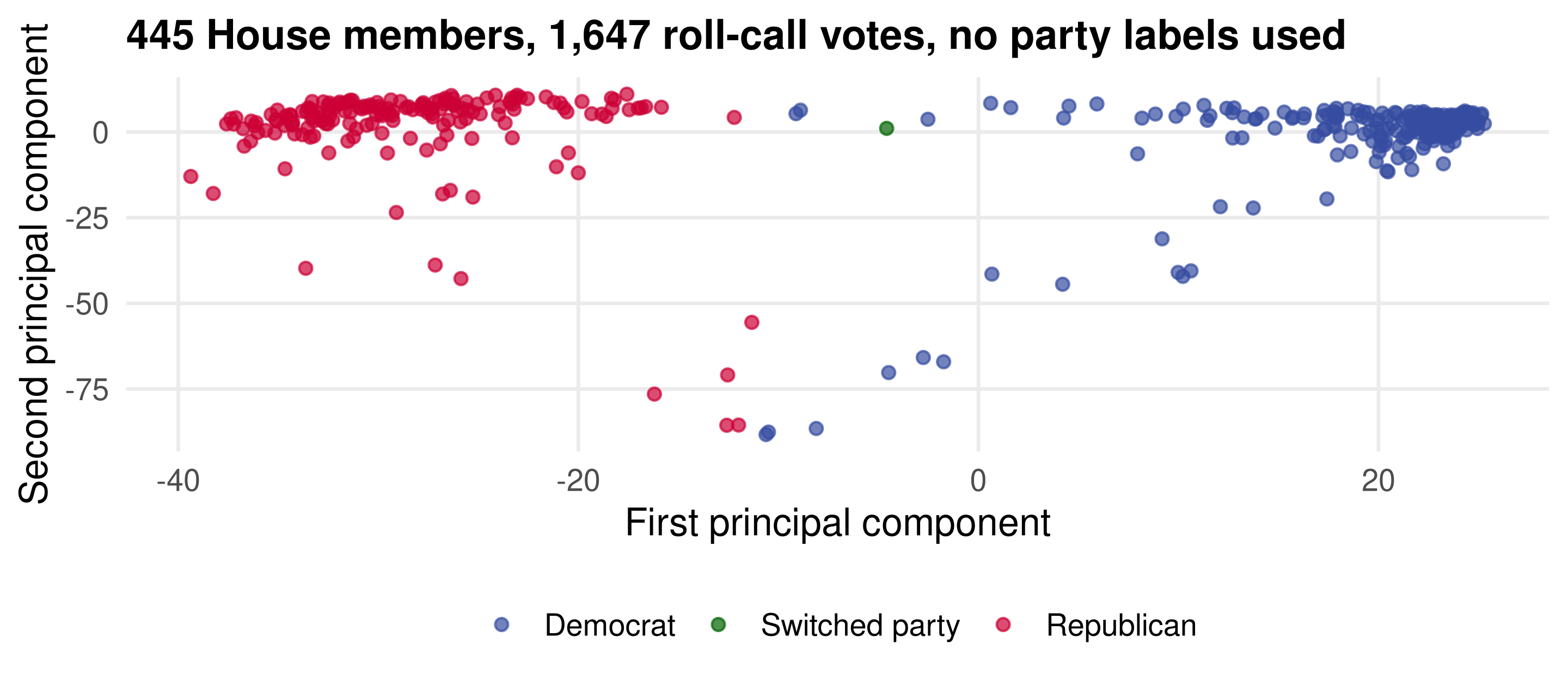
• Each member is a point in 1,647 dimensions: yea, nay or abstain on every vote of the 111th Congress.
• Principal component analysis found the direction of greatest disagreement without being told the parties. The colours were added afterwards.
• Who are the members trailing off the bottom? Section 4 finds out.

The axis along which members differ most is the party line, so the first component is an ideology score; the parties are told apart by sign alone for 435 of 445 members. The second component surprises: it is attendance, not ideology. Both are explained in section 4 with the code.

Today’s route

1. Learning without labels: what changes when there is no Y, and two latent-variable models that organize the lecture.
2. K-means clustering: the mixture model, the algorithm, its local minima, and European diets.
3. Principal component analysis: the linear factor model, the singular value decomposition, loadings, scores and scree plots.
4. PCA in the wild: Congress in two dimensions and the business cycle in one.
5. Principal components regression: factors as regressors, and the online spending data of lecture 12 revisited.

Additional derivations and code follow the main lesson.

Lectures 11 to 13 estimated E[Y | X] with an out-of-sample objective to keep us honest. Today there is no Y, so there is no out-of-sample error to minimize; the objective is to describe X with fewer numbers than it has. The two tools, K-means and PCA, are the two ways of doing that: group the observations, or rotate the coordinates.

Packages and data

Run the examples from the lectures/ directory.

library(tidyverse)
library(patchwork)   # side-by-side ggplots
library(Matrix)      # the sparse browsing matrix of lecture 12
library(glmnet)      # the lasso, for the comparison in section 5

kmeans() and prcomp() are in base R; no package is needed for the methods themselves.

File	Role
data/protein.csv	Protein consumption of 25 European countries in nine food groups
data/rollcall-votes.csv, data/rollcall-members.csv	1,647 roll-call votes of the 445 members of the 111th House
data/2024-07-fredmd.csv	FRED-MD, 126 monthly US macroeconomic series since 1959
data/browser-totalspend.csv, data/browser-domains.csv, data/browser-sites.txt	Online spending and browsing of 10,000 households

[Sources] - The protein data (Weber 1973) and the roll-call data accompany Taddy, Business Data Science (2019), chapter 7; the notes use the protein data and keep the roll-call application in a comment. - FRED-MD is McCracken and Ng (2016), downloaded from the St. Louis Fed; lecture 17 uses the same file. - The browser data are the comScore panel of lecture 12.

Learning without labels

---

What changes when there is no Y

Supervised learning, lectures 11 to 13

• Data (X_i, Y_i); target \mathbf{E}[Y \mid X].
• Regularization found a low-dimensional regression function inside a high-dimensional X.
• A clear objective: predict Y_{n+1} from X_{n+1}, judged out of sample.

Unsupervised learning, today

• Data X_i only, usually high-dimensional.
• Posit a simpler structure that generates X and learn that structure.
• The goal is to simplify X for its own sake, or to feed the simplified X into a later prediction.

Two methods: K-means clustering groups the observations; principal component analysis finds the few directions along which they vary.

Regularization in lectures 12 and 13 was a tool for a supervised goal. Today the dimension reduction is the goal. The two methods correspond to two different latent-variable models, which is the thread of the lecture.

What is it used for

• Seeing the data. Twenty-five countries in nine food groups cannot be plotted; two principal components can.
• Grouping. Cluster shoppers by purchases, voters by their issues, Spotify users by taste. Clustering can be exploratory, like a histogram, or operational: a recommendation engine recommends what similar users watched.
• Few labels, many observations. Thousands of tweets, a few hand-labelled for sentiment: cluster the tweets by topic, then let the labelled tweets in each topic predict the rest.
• Preprocessing for prediction. Replace a thousand correlated regressors by a handful of factors, then run a regression. That is section 5.

The last use is the bridge back to supervised learning: PCA produces regressors, and the regression is then ordinary. The first three uses are where unsupervised learning stands on its own.

Two latent-variable models organize the lecture

	Mixture model	Linear factor model
Hidden variable	A type C_i \in \{1, \dots, K\}	K continuous factors Z_{i1}, \dots, Z_{iK}
Observed X_i	A draw from the type’s distribution f_{C_i}	\mu + Z_{i1}\varphi_1 + \dots + Z_{iK}\varphi_K + \varepsilon_i
What we learn	Which type each observation is	The directions \varphi_k and each observation’s scores Z_{ik}
Method	K-means	Principal component analysis
Picture	K clouds of points	A K-dimensional plane through the cloud

In both, X is d-dimensional and the hidden variable has K \ll d pieces. A discrete hidden variable gives clusters; a continuous one gives a plane.

Keep this table in mind: every later slide fills one of its cells. The mixture model is in Hastie, Tibshirani and Friedman section 14.3; the factor model and PCA in section 14.5.

A word of caution

Warning

With supervised learning, a story about X that did not help predict Y out of sample was dropped. With unsupervised learning, there is no Y_{n+1} to check against, so it is easy to “discover” structure that is not there.

• A multimodal histogram may be one distribution, not a mixture of several.
• A cluster can be an artifact of the scale of the variables, the number K we chose, or the random start.
• A principal component picks up the largest source of variation, whatever it is. In section 4 that turns out to be attendance.

The discipline has to come from us: replicate across starts, check the scale, interpret with care.

This is the paragraph the notes leave in a comment. It matters: the methods always return K clusters and K components, whether or not the data have them.

K-means clustering

---

The mixture model

Model the distribution f of the data X as a weighted sum of K distributions,

f(x) = \pi_1 f_1(x) + \dots + \pi_K f_K(x), \qquad \pi_k \ge 0, \quad \sum_{k=1}^K \pi_k = 1.

• f_1, \dots, f_K are the mixture components; \pi_1, \dots, \pi_K the mixture weights.

The same model with a hidden variable. Let U_k \sim f_k for k = 1, \dots, K. To draw X:

1. draw a type C with \Pr(C = k) = \pi_k;
2. set X = U_C.

Only X is observed. The type C is latent, and recovering it is the clustering problem.

The two descriptions are the same distribution: integrate out C and the density is the weighted sum. The second one is what the algorithm will imitate: guess each observation’s type, describe each type, repeat.

Example: types of shoppers

• X_i is a vector of one shopper’s purchases on Amazon in a month, one component per item.
• Suppose there are K latent types: a new parent who buys baby items, someone who buys mainly electronics, and so on.
• The component f_k describes the purchases of type k across all items.
• The weight \pi_k is the share of shoppers who are type k.

The analyst never sees the types. From a large dataset of purchases, K-means tries to recover them: which shoppers are of the same type, and what does each type buy?

A type is a cluster, a mixture component is what a cluster looks like, and a mixture weight is a cluster’s size. The protein data later make this concrete with countries as shoppers and food groups as items.

What a mixture looks like in one dimension

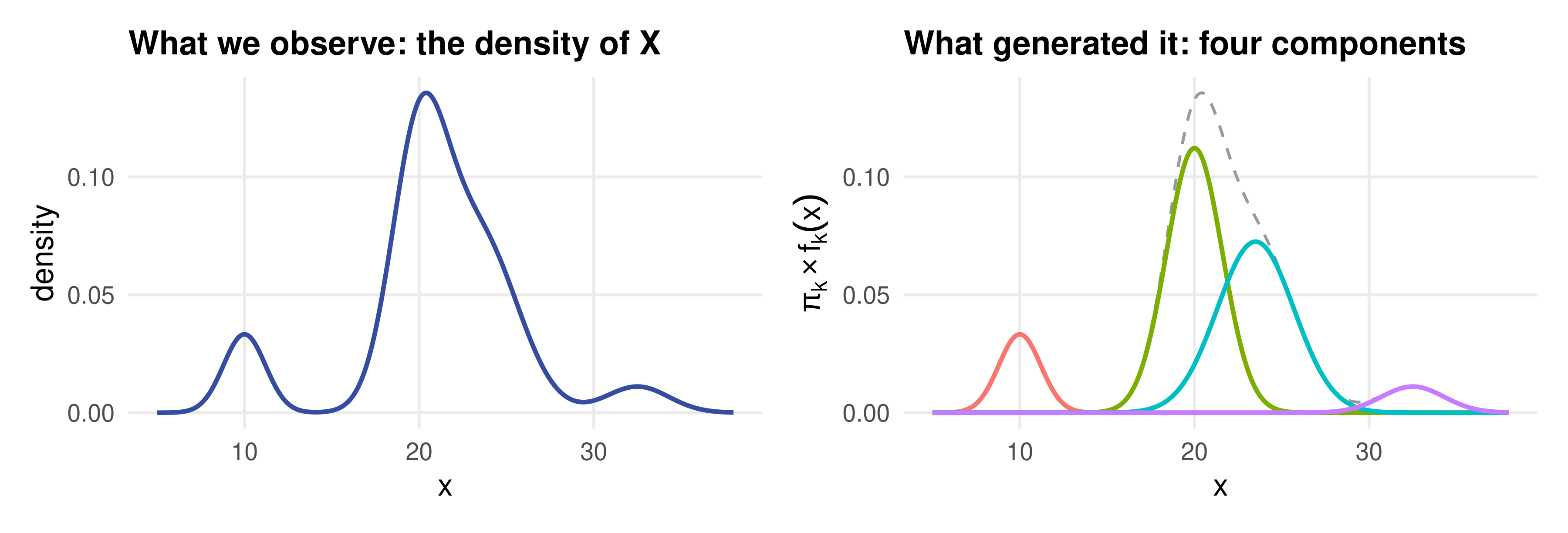
• Left: the density of X. Right: the four normal components, each scaled by its weight, that add up to it.
• The weights here are 0.10, 0.45, 0.40 and 0.05. The two middle components overlap, so an X near 22 could have come from either.

The notes show the same picture as two static images. The overlap in the middle is the point: cluster membership is uncertain where components overlap, and K-means will nonetheless draw a hard boundary there.

From mixtures to K-means

• The picture on the left could also be a single distribution with four modes. To estimate a mixture we must say more about the components.
• The usual assumption is normality, U_k \sim N(\mu_k, \sigma_k^2): the Gaussian mixture model, estimated by maximum likelihood with the EM algorithm, because the likelihood is not concave.

K-means is the simpler method we cover. It keeps the latent-type structure and drops the likelihood:

• each type is summarized by its centre \mu_k;
• each observation belongs to the type whose centre is closest.

Formally, K-means is the Gaussian mixture in the limit \sigma_k^2 \to 0 for every k (Hastie, Tibshirani and Friedman, section 14.3.7; the appendix sketches why).

With a vanishing variance, the posterior probability that an observation belongs to the nearest centre goes to one, so the soft EM assignments become the hard assignments of K-means. The price is that K-means cannot express uncertainty about membership.

The K-means algorithm

Given data X_1, \dots, X_n with X_i = (X_{i1}, \dots, X_{id})' and a number of groups K:

1. Start. Draw initial memberships \hat C_1, \dots, \hat C_n \in \{1, \dots, K\} at random.
2. Centres. For each group, the average of its members, \hat\mu_k = \frac{\sum_{i=1}^n X_i\, \mathbf{1}\{\hat C_i = k\}}{\sum_{i=1}^n \mathbf{1}\{\hat C_i = k\}}.
3. Reassign. Move each observation to the group whose centre is nearest, \hat C_i = \arg\min_k \sum_{j=1}^d (X_{ij} - \hat\mu_{kj})^2.
4. Repeat steps 2 and 3 until no membership changes.

This is Lloyd’s algorithm. The next two slides run it by hand on simulated data so that every step is visible; R’s kmeans() uses a refinement, Hartigan and Wong’s, discussed after the application.

The algorithm in eight lines

set.seed(2)                                               # three clouds of 50 points
X <- matrix(c(-2, 0, 2, 1.5, -2, 0.5), ncol = 2)[rep(1:3, each = 50), ] +
  matrix(rnorm(300, sd = 0.8), ncol = 2)
K <- 3
set.seed(12); C <- sample(1:K, nrow(X), replace = TRUE)    # step 1: random labels
repeat {
  mu <- t(sapply(1:K, function(k) colMeans(X[C == k, , drop = FALSE])))   # step 2: centres
  d2 <- sapply(1:K, function(k) colSums((t(X) - mu[k, ])^2))             # squared distances
  C_new <- apply(d2, 1, which.min)                                        # step 3: reassign
  if (all(C_new == C)) break                                              # step 4: until stable
  C <- C_new
}
c(within_SS = sum(d2[cbind(1:nrow(X), C)]), kmeans = kmeans(X, centers = 3, nstart = 10)$tot.withinss)

## within_SS    kmeans 
##  206.3774  206.3774

The hand-written loop and kmeans() reach the same partition and the same within-cluster sum of squares.

d2 is an n by K matrix of squared distances from each point to each centre; d2[cbind(1:n, C)] picks each point’s distance to its own centre. The sum is the objective of the next slide.

Watching it converge

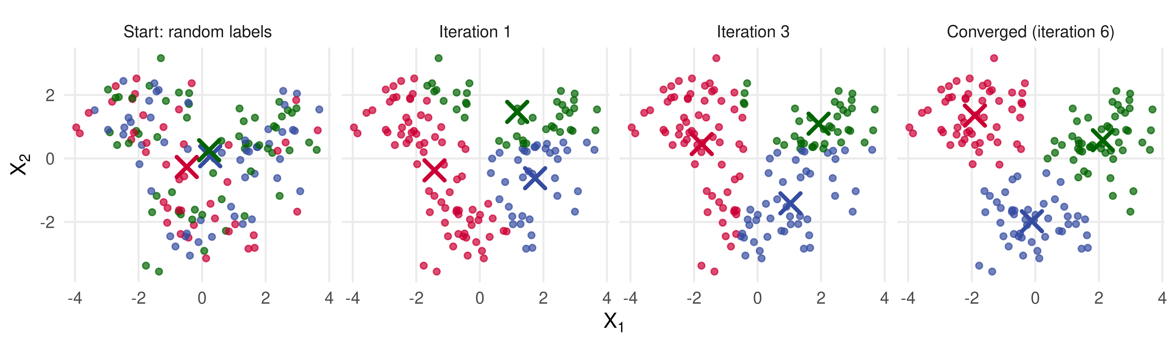
• Random labels put all three centres in the middle of the data. One pass pulls them apart; a few more passes settle the boundary points.
• Crosses mark the centres \hat\mu_k at the start of each iteration.

Iteration counts depend on the start: with other seeds this data set converges in two to six passes. The three clouds are well separated, so every start we tried reached the same partition; the protein data below will not be so kind.

What K-means minimizes

Steps 2 and 3 are coordinate descent on the within-cluster sum of squares,

W(\hat C, \hat\mu) = \sum_{i=1}^n \sum_{j=1}^d (X_{ij} - \hat\mu_{\hat C_i, j})^2 = \sum_{k=1}^K \sum_{i:\, \hat C_i = k} \lVert X_i - \hat\mu_k \rVert^2.

• Step 2 minimizes W over the centres for fixed memberships: the minimizer of a sum of squares is the mean.
• Step 3 minimizes W over the memberships for fixed centres.
• W never increases, and there are finitely many partitions, so the loop stops. R calls W tot.withinss; the notes call it the deviance.

Warning

It stops at a local minimum. The problem is not convex, the global minimum is NP-hard, and different random starts can end at different partitions.

The appendix gives the two-line proof of monotonicity and the pairwise-distance form of W. The nonconvexity is the practical headache: it is why every call below sets nstart.

Application: diets in (former) European countries

Protein consumption in grams per person per day, 25 countries, nine food groups (Weber 1973).

food <- read.csv("data/protein.csv", row.names = 1)
dim(food)

## [1] 25  9

head(food, 6)

##                RedMeat WhiteMeat Eggs Milk Fish Cereals Starch Nuts Fr.Veg
## Albania           10.1       1.4  0.5  8.9  0.2    42.3    0.6  5.5    1.7
## Austria            8.9      14.0  4.3 19.9  2.1    28.0    3.6  1.3    4.3
## Belgium           13.5       9.3  4.1 17.5  4.5    26.6    5.7  2.1    4.0
## Bulgaria           7.8       6.0  1.6  8.3  1.2    56.7    1.1  3.7    4.2
## Czechoslovakia     9.7      11.4  2.8 12.5  2.0    34.3    5.0  1.1    4.0
## Denmark           10.6      10.8  3.7 25.0  9.9    21.9    4.8  0.7    2.4

Each country is a point in nine dimensions. K-means groups countries with similar diets, so a cluster is, roughly, a diet.

Row names are the countries, so the data frame has nine numeric columns. The country names reflect the early 1970s: USSR, Czechoslovakia, East and West Germany, Yugoslavia.

Scale first

Squared distance adds up the columns, so a column measured in big numbers dominates. The standard deviations differ by a factor of ten:

round(apply(food, 2, sd), 1)

##   RedMeat WhiteMeat      Eggs      Milk      Fish   Cereals    Starch      Nuts    Fr.Veg 
##       3.3       3.7       1.1       7.1       3.4      11.0       1.6       2.0       1.8

Standardize every column, as with the lasso: centre at the mean, divide by the standard deviation. A unit of xfood is one standard deviation.

xfood <- scale(food)

Without scaling, cereals (sd 11) and milk (sd 7) would decide the clusters on their own and eggs (sd 1.1) would be irrelevant. Scaling is a modelling choice, not a technicality: it says every food group matters equally.

kmeans() with three diets

set.seed(0)
grpMeat <- kmeans(xfood, centers = 3, nstart = 10)   # centers = K; nstart = random starts
grpMeat$size

## [1]  6 15  4

round(grpMeat$centers, 2)

##   RedMeat WhiteMeat  Eggs  Milk  Fish Cereals Starch  Nuts Fr.Veg
## 1   -0.79     -0.53 -1.17 -0.90 -0.95    1.44  -0.76  0.89  -0.54
## 2    0.45      0.51  0.58  0.58  0.12   -0.61   0.35 -0.70  -0.22
## 3   -0.51     -1.11 -0.41 -0.83  0.98    0.13  -0.18  1.31   1.63

• centers = 3 asks for K = 3 groups; nstart = 10 runs the algorithm from ten random starts and keeps the lowest W.
• $centers holds \hat\mu_k in standard deviation units: cluster 1 eats 1.4 sd more cereals than average and 1.2 sd fewer eggs.

Cluster numbers are arbitrary labels; another seed can permute them. What is stable, if the minimum is found, is the partition.

Who is in each cluster

split(names(grpMeat$cluster), grpMeat$cluster)

## $`1`
## [1] "Albania"    "Bulgaria"   "Hungary"    "Romania"    "USSR"       "Yugoslavia"
## 
## $`2`
##  [1] "Austria"        "Belgium"        "Czechoslovakia" "Denmark"        "E Germany"     
##  [6] "Finland"        "France"         "Ireland"        "Netherlands"    "Norway"        
## [11] "Poland"         "Sweden"         "Switzerland"    "UK"             "W Germany"     
## 
## $`3`
## [1] "Greece"   "Italy"    "Portugal" "Spain"

c(within_SS = grpMeat$tot.withinss, between_share = grpMeat$betweenss / grpMeat$totss)

##     within_SS between_share 
##   105.9863300     0.5093225

• Cluster 1: the Balkans, Hungary and the USSR; cereals and nuts.
• Cluster 2: Western, Northern and Central Europe; meat, eggs and milk.
• Cluster 3: Greece, Italy, Portugal and Spain; fish, fruit and vegetables. The three centres account for 51 percent of the total sum of squares.

The between-cluster share is R squared for a regression of xfood on cluster dummies. Czechoslovakia, East Germany and Poland join the Western cluster: their diets in 1973 were closer to Austria’s than to Romania’s.

The clusters on a map of two food groups

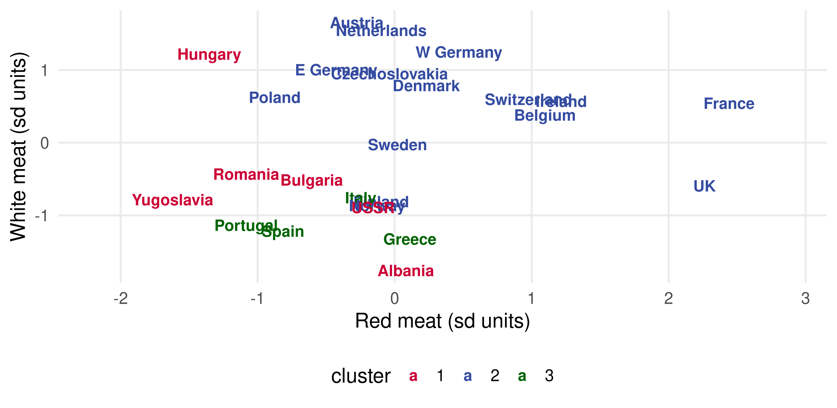
Two of the nine dimensions, chosen for the plot; the clusters were found in all nine. The Western cluster spans the whole range of white meat, so this pair of axes does not separate it from the others on its own.

The notes draw this with base graphics and text(). Any two columns of xfood can be plotted; red meat against fish is the next useful pair and appears after the seven-cluster fit.

Different starts, different answers

Twenty runs from a single random start each, same data, same K = 3:

set.seed(1)
single <- replicate(20, kmeans(xfood, centers = 3, nstart = 1)$tot.withinss)
table(round(single, 1))

## 
##   106 106.4 114.7 120.5 121.8 
##     8     2     7     2     1

• Only 8 of the 20 runs find the partition with W = 106.0; the others stop at local minima up to 15 percent worse.
• Always set nstart, ten or more, and keep the run with the smallest W. kmeans() does this for you.
• kmeans() also refines steps 2 and 3: Hartigan and Wong’s algorithm checks whether moving any single observation lowers W, which escapes some local minima that plain reassignment cannot.

Every run here has the same objective and the same data; only the random first labels differ. The run with W = 106.0 is the one grpMeat found with nstart = 10.

Seven diets

set.seed(0)
grpProtein <- kmeans(xfood, centers = 7, nstart = 50)
split(names(grpProtein$cluster), grpProtein$cluster)

## $`1`
## [1] "Czechoslovakia" "Hungary"        "Poland"         "USSR"          
## 
## $`2`
## [1] "Portugal" "Spain"   
## 
## $`3`
## [1] "Albania"    "Bulgaria"   "Romania"    "Yugoslavia"
## 
## $`4`
## [1] "Denmark" "Finland" "Norway"  "Sweden" 
## 
## $`5`
## [1] "Belgium"     "France"      "Ireland"     "Switzerland" "UK"         
## 
## $`6`
## [1] "Greece" "Italy" 
## 
## $`7`
## [1] "Austria"     "E Germany"   "Netherlands" "W Germany"

A finer subdivision of the three blocks, and the subdivisions are familiar: Scandinavia, the British Isles with France, Belgium and Switzerland, the German-speaking centre, the Iberian peninsula, and so on.

With K = 7 the 25 countries fall into groups of two to five, each a recognizable cultural or geographic region. Nothing about geography went in; only grams of protein.

Seven clusters, two views

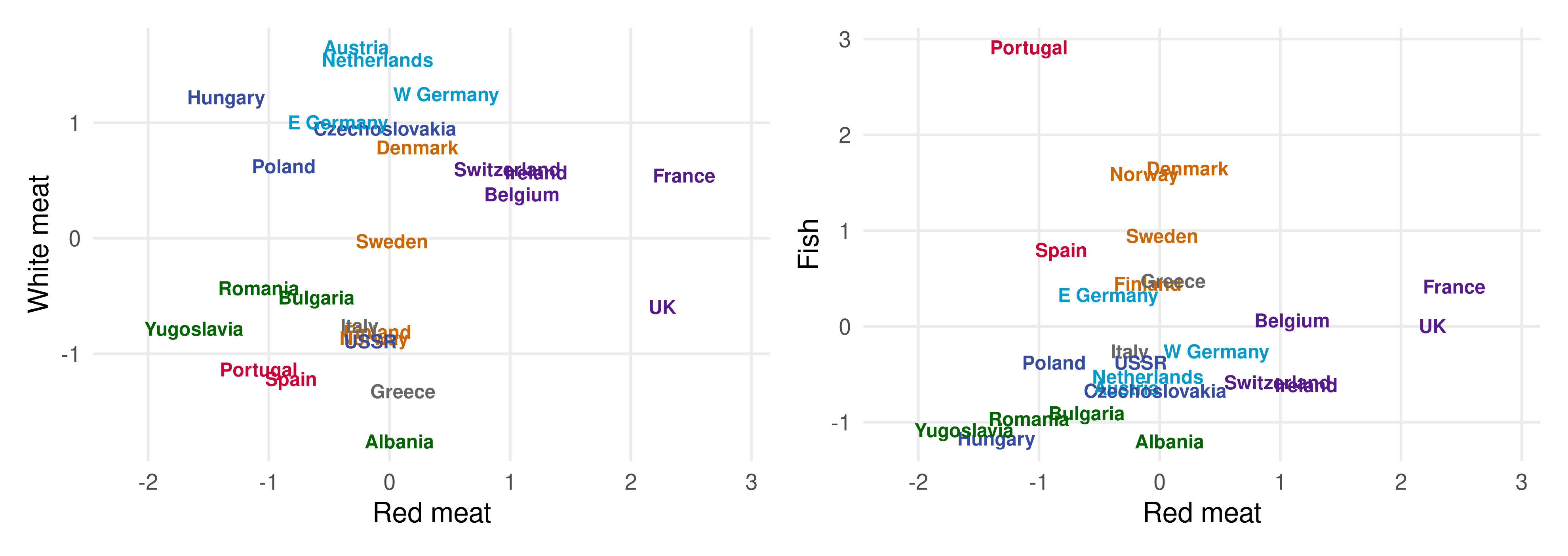
• Same clusters, two pairs of axes. Red meat against fish separates the Iberian pair and the Scandinavians, which the white meat axis hid.
• No two-dimensional plot shows a nine-dimensional partition faithfully. Section 3 builds a better pair of axes.

The best two axes for displaying the clusters are not any two food groups but the first two principal components, which is the natural segue into PCA.

Choosing K

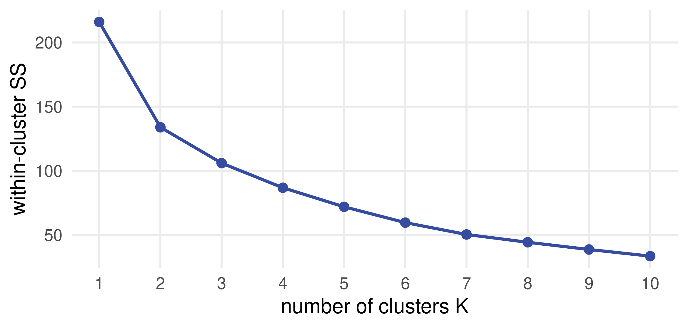
• W always falls with K and reaches zero at K = n, so it cannot choose K. Practitioners look for an “elbow”; there is none here.
• With supervised learning, cross-validation chose the complexity. Here there is no out-of-sample prediction to check, so the choice of K is a matter of interpretation: what counts as a diet? Movie genres, or sub-genres?

The notes’ answer is the honest one: K is subjective. There are formal criteria (the gap statistic, silhouettes), but they encode a definition of “cluster” rather than discover one. With K = 3 we got three macro-regions; with K = 7 seven recognizable regions. Both are useful descriptions.

Checkpoint: K-means

1. The algorithm is run twice with different random starts and returns different partitions. Which one should you report, and how would you know?
2. Why does kmeans() on unscaled protein data put almost all the weight on cereals and milk?
3. A friend runs K-means with K = 25 on the 25 countries and reports W = 0. What went wrong?

Answers: the one with the lower within-cluster sum of squares, read from tot.withinss; better, use nstart so that kmeans() does the comparison. Squared Euclidean distance sums squared differences across columns, and cereals and milk have standard deviations of 11 and 7 grams against 1 or 2 for eggs, nuts and starch, so they dominate the sum. Each country is its own cluster; W falls to zero at K = n by construction, which is why W cannot choose K.

Principal component analysis

---

The linear factor model

K-means put a d-dimensional X_i into one of K boxes. A linear factor model instead writes it as a combination of K unobserved numbers:

\underbrace{X_i}_{d \times 1} = \mu + \underbrace{Z_{i1}}_{1 \times 1}\underbrace{\varphi_1}_{d \times 1} + \dots + \underbrace{Z_{iK}}_{1 \times 1}\underbrace{\varphi_K}_{d \times 1} + \varepsilon_i.

• Z_{ik} is a scalar factor (or score): how much of pattern k observation i has.
• \varphi_k is a d-vector of factor loadings: what pattern k looks like across the d variables.

It looks like a regression of X_i on Z_i, but

• the outcome X_i is d-dimensional, not a scalar Y_i;
• the “regressors” Z_{i1}, \dots, Z_{iK} are unobserved. We estimate both the regressors and the coefficients.

For the diets, a factor might be “animal versus plant protein” with a loading vector that is negative on meat, eggs and milk and positive on cereals and nuts; each country’s score says where it sits on that axis.

The PCA objective

Both Z and \varphi are unknown, so the model needs normalizations, just as a mixture needed a shape for its components. Principal component analysis picks \hat Z and \hat\varphi to minimize

\sum_{i=1}^n \sum_{j=1}^d \big(X_{ij} - \bar X_j - Z_{i1}\varphi_{1j} - \dots - Z_{iK}\varphi_{Kj}\big)^2

subject to

• the factors Z_{\cdot 1}, \dots, Z_{\cdot K} being uncorrelated across i;
• the loadings being orthonormal: \varphi_j'\varphi_k = 0 for j \ne k and \varphi_k'\varphi_k = 1.

• Order the factors by decreasing sample variance. The ordered pairs (\hat Z_{\cdot k}, \hat\varphi_k) are the principal components.
• Reading PCA as the estimate of a “true” factor model needs more (uncorrelated \varepsilon_{ij}); as a description of the data it needs nothing more.

Without the normalizations the problem has no unique answer: multiply Z by two and divide phi by two, or rotate both. Orthonormal loadings and uncorrelated factors pin down the solution up to the sign of each component.

The geometry in two dimensions

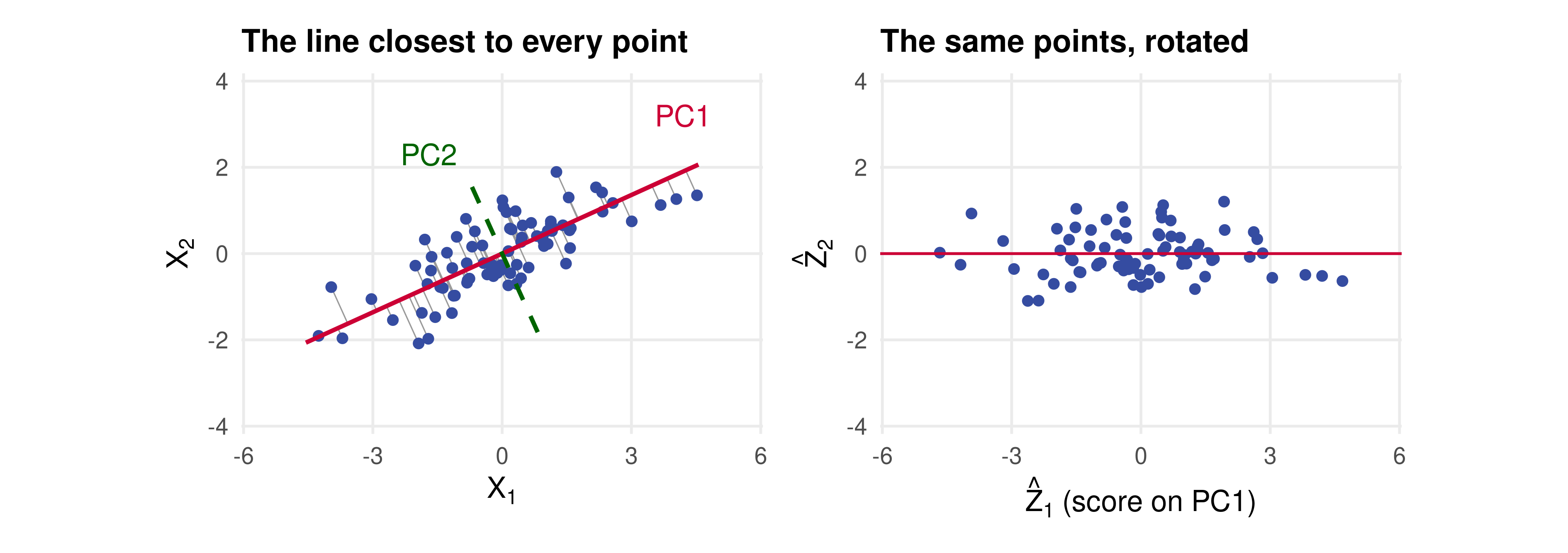
• d = 2, K = 1: PCA finds the line through the centred cloud that minimizes the squared perpendicular distances. The grey segments are the residuals \varepsilon_i; the score \hat Z_{i1} is where the foot of each segment lands.
• Equivalently, PC1 is the direction along which the projected points have the largest variance. PC2 is the perpendicular direction, and the rotated coordinates on the right are uncorrelated.

Minimum reconstruction error and maximum projected variance are the same problem by Pythagoras: the squared length of each point is its squared projection plus its squared residual, and the first is fixed by the data. The appendix has the derivation.

In three dimensions

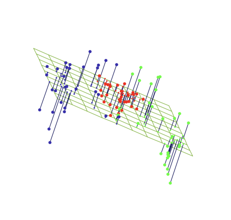
With d = 3 and K = 2, PCA fits a plane through the cloud.

• \hat\varphi_1 and \hat\varphi_2 span the plane; (\hat Z_{i1}, \hat Z_{i2}) are observation i’s coordinates on it.
• The segments are the residuals \varepsilon_i, perpendicular to the plane.
• In general PCA finds the K-dimensional subspace closest to the d-dimensional cloud, and approximates each observation by \bar X + \hat Z_{i1}\hat\varphi_1 + \dots + \hat Z_{iK}\hat\varphi_K.

Colours in the picture are three clusters, to make the point that points which cluster in d dimensions usually still cluster on the fitted plane, which is why the components make good axes for displaying K-means results.

Computing it: the singular value decomposition

Let X be the n \times d matrix of centred (and scaled) data. Linear algebra factors it as

\underbrace{X}_{n \times d} = \underbrace{U}_{n \times n}\;\underbrace{D}_{n \times d}\;\underbrace{V'}_{d \times d},

with U'U = I_n, V'V = I_d, and D zero off the diagonal with weakly decreasing diagonal entries d_1 \ge d_2 \ge \dots.

• The kth loading vector \hat\varphi_k is the kth column of V.
• The kth factor \hat Z_{\cdot k} is the kth column of UD, which equals X\hat\varphi_k: the data projected onto the kth loading.
• The sample variance of \hat Z_{\cdot k} is d_k^2/(n - 1), decreasing in k by construction.

The kth component does not depend on K. Fitting one factor or five gives the same \hat\varphi_1 and \hat Z_{\cdot 1}, so “the first principal component” is well defined.

R’s prcomp() calls svd(). The appendix checks every claim here numerically on the protein data. The nesting property is special to PCA; K-means with K = 3 and K = 7 shares nothing.

prcomp() on the European diets

pcfood <- prcomp(food, center = TRUE, scale = TRUE, rank = 5)   # rank = K; centre and scale as before
round(pcfood$rotation, 2)   # loadings: column k is the kth principal component

##             PC1   PC2   PC3   PC4   PC5
## RedMeat   -0.30 -0.06 -0.30 -0.65  0.32
## WhiteMeat -0.31 -0.24  0.62  0.04 -0.30
## Eggs      -0.43 -0.04  0.18 -0.31  0.08
## Milk      -0.38 -0.18 -0.39  0.00 -0.20
## Fish      -0.14  0.65 -0.32  0.22 -0.29
## Cereals    0.44 -0.23  0.10  0.01  0.24
## Starch    -0.30  0.35  0.24  0.34  0.74
## Nuts       0.42  0.14 -0.05 -0.33  0.15
## Fr.Veg     0.11  0.54  0.41 -0.46 -0.23

• center and scale standardize the columns as scale() did for K-means.
• rank = 5 keeps five components. Because of nesting, the first two columns would be identical with rank = 2.

The sign of each column is arbitrary: prcomp() could return the negative of any column and the fit would be identical. Interpretations must survive a sign flip, which they do if we read the signs relative to each other.

Reading the loadings

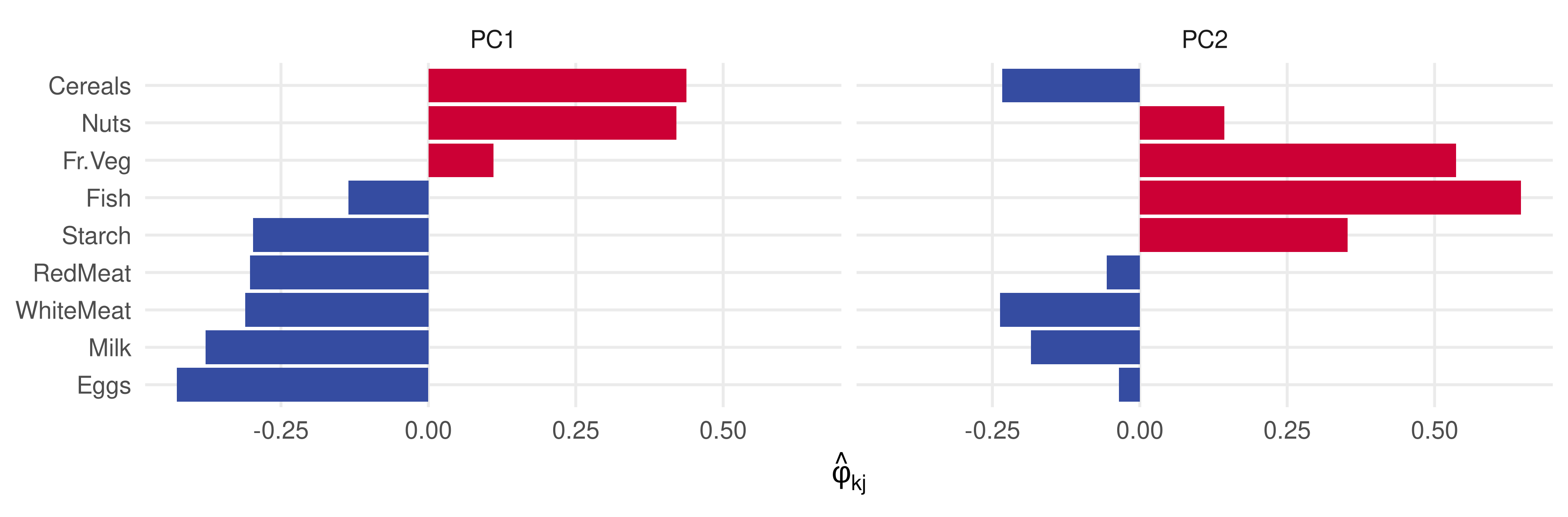
• Each X_{ij} is in standard deviation units, so \hat\varphi_{kj} is the rise in food group j, in standard deviations, per unit of factor k.
• PC1: positive on cereals and nuts, negative on meat, eggs and milk: plant versus animal protein, plausibly wealth. Starch goes against the story.
• PC2: fish, fruit and vegetables, starch: a Mediterranean diet? PC3 loads on white meat; PC4 and PC5 are harder to read.

Both bar charts are drawn from pcfood$rotation. The interpretation of PC1 is the one the notes propose, with the same caveat about starch. Higher components are usually harder to interpret, which is one reason to stop early.

The scores: each country on each component

predict() returns the n \times K matrix of factors \hat Z_{ik}.

food_factors <- predict(pcfood)
round(head(food_factors, 4), 2)

##            PC1   PC2   PC3   PC4   PC5
## Albania   3.49 -1.63 -1.76 -0.23  0.02
## Austria  -1.42 -1.04  1.34 -0.17 -0.93
## Belgium  -1.62  0.16  0.22 -0.52  0.76
## Bulgaria  3.13 -1.30  0.15 -0.21 -0.48

round(sort(food_factors[, 1]), 1)[c(1:4, 22:25)]      # the ends of PC1

##    Ireland    Denmark  W Germany         UK    Romania   Bulgaria    Albania Yugoslavia 
##       -2.7       -2.4       -2.1       -1.7        2.8        3.1        3.5        3.6

round(sort(food_factors[, 2], decreasing = TRUE), 1)[1:3]   # the top of PC2

## Portugal    Spain   Greece 
##      4.3      2.6      1.0

• PC1 is negative for Ireland, Denmark, West Germany and the UK, positive for the Balkans: the east-west, animal-plant division. PC2 is largest for Portugal and Spain, then Greece: the Mediterranean reading survives.

The scores are read against the loadings: a country with a large positive PC1 has more cereals and nuts and less meat than average. Check it against Albania’s row in the raw data: 42 grams of cereal protein against an average of 32, and 1.4 grams of white meat against 7.9.

Countries in principal component space

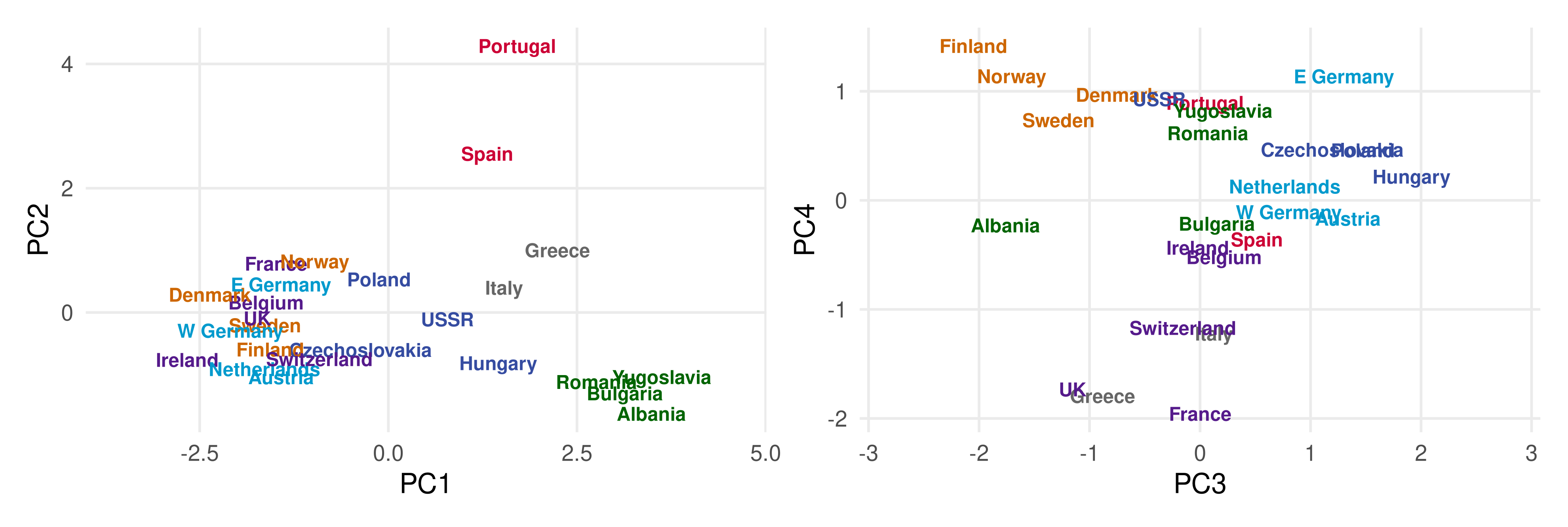
• Colours are the seven K-means clusters. On PC1 and PC2 the clusters sit apart: countries that K-means grouped are close in component space, although neither method saw the other.
• PC3 against PC4 carries little of the structure. Two components were the right axes; two food groups were not.

This is the promised better pair of axes. The agreement between K-means and PCA is not guaranteed; it says the dominant variation in these data is between groups rather than within them.

How many components? The scree plot

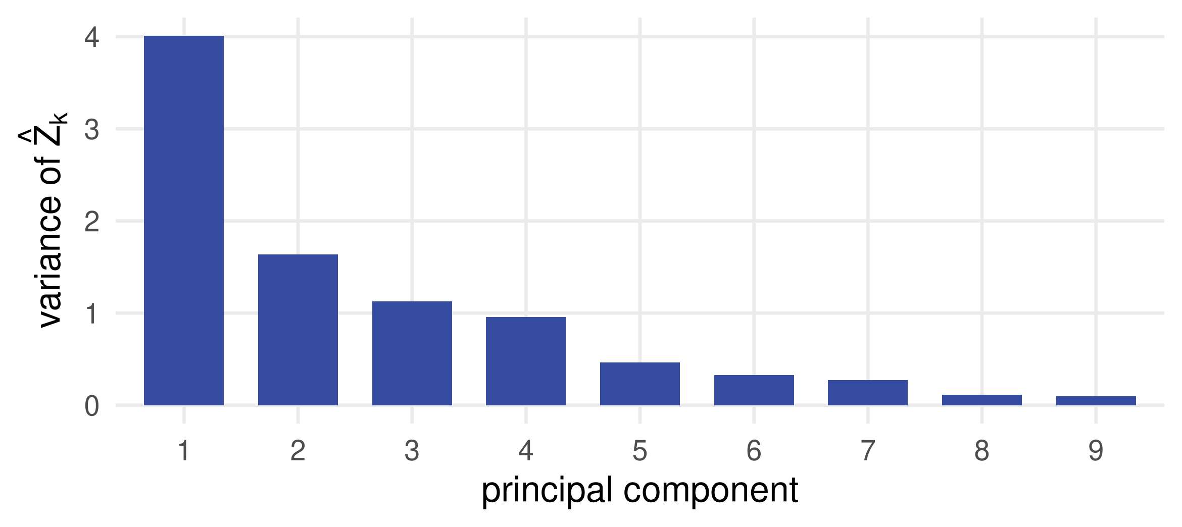
• The variance of \hat Z_{\cdot k} falls with k by construction. Under a “true” factor model with K_0 factors, it should drop to about zero after K_0.
• Here there is a drop after the first component and another after the fourth. One factor, or four? The notes’ plot(pcfood) draws the same bars.

Scree is the rubble at the foot of a cliff: the small components after the drop are supposed to be noise. On nine food groups and 25 countries the picture is suggestive at best.

Proportion of variance explained

summary(pcfood)

## Importance of first k=5 (out of 9) components:
##                           PC1    PC2    PC3    PC4     PC5
## Standard deviation     2.0016 1.2787 1.0620 0.9771 0.68106
## Proportion of Variance 0.4452 0.1817 0.1253 0.1061 0.05154
## Cumulative Proportion  0.4452 0.6268 0.7521 0.8582 0.90976

• The variances sum to d = 9 after scaling, so the share of component k is \hat{\operatorname{Var}}(\hat Z_{\cdot k})/9: 45 percent for PC1, 63 percent for the first two, 86 percent for four.
• The share is the proportional fall in the PCA objective from adding the component, like the explained sum of squares in an in-sample R^2, with the same two warnings: it is in-sample, and a large share does not certify a “true” factor.

Nine components explain everything, trivially, just as a regression with n parameters fits perfectly. The cumulative row is the one people quote; the right number of components to quote is the one you can interpret.

Choosing K for PCA

• As with clustering, K is a matter of interpretation, not of a prediction loss.
• Nesting helps: compute a large K once, then read the components in order and stop when they stop making sense. For the diets that is two, perhaps three.
• The scree plot and the variance shares guide the eye. In economics, Bai and Ng (2002) turn the drop in the scree plot into an information criterion for the number of factors.
• For principal components regression, section 5, K becomes a tuning parameter with an out-of-sample criterion again, and cross-validation returns.

The difference from supervised learning is the absence of a loss defined by the task. The moment a task appears, as in section 5, the usual machinery applies.

Checkpoint: PCA

1. The loadings of PC1 are multiplied by -1 and so are its scores. Has anything changed?
2. Why does prcomp(food, rank = 2) give the same first two loadings as rank = 5, when kmeans() with K = 3 and K = 7 gives unrelated clusters?
3. The first two components explain 63 percent of the variance of the scaled protein data. What would the share be if scale = FALSE and why would it be misleading?

Answers: nothing; the fit and the sum of squares are identical, only the sign convention differs, so read loadings and scores together. PCA’s components come from one singular value decomposition and are nested; K-means re-solves a different combinatorial problem for each K. Without scaling, cereals with variance 120 would dominate the total variance of about 230, so one component would explain most of it by reproducing the cereal column, which says nothing about diets as a whole.

PCA in the wild

---

Congress in two dimensions, the business cycle in one

Roll-call votes in the 111th House

votes <- read.csv("data/rollcall-votes.csv")
legis <- read.csv("data/rollcall-members.csv")
dim(votes)

## [1]  445 1647

votes[1:4, 1:5]        # -1 nay, +1 yea, 0 abstained

##                   Vote.1 Vote.2 Vote.3 Vote.4 Vote.5
## BONNER (R AL-1)       -1      1     -1      0      0
## BRIGHT (D AL-2)        1     -1      1      1      1
## ROGERS (R AL-3)       -1      1     -1     -1     -1
## ADERHOLT (R AL-4)     -1      1     -1     -1      1

table(legis$party)

## 
##   D  DR   R 
## 262   1 182

Every recorded vote of 2009 and 2010: 445 members, 1,647 votes. Is there a low-dimensional structure in a member’s 1,647 votes? One candidate factor is obvious: ideology.

The 445 exceed the 435 seats because of mid-term replacements. “DR” marks a member who switched party during the Congress (Parker Griffith of Alabama).

One dominant factor

pcavote <- prcomp(votes, scale = TRUE)   # K not chosen yet: all 445 components
round(100 * summary(pcavote)$importance[2, 1:6], 1)   # percent of variance

##  PC1  PC2  PC3  PC4  PC5  PC6 
## 36.4 13.0  3.4  2.5  1.2  1.1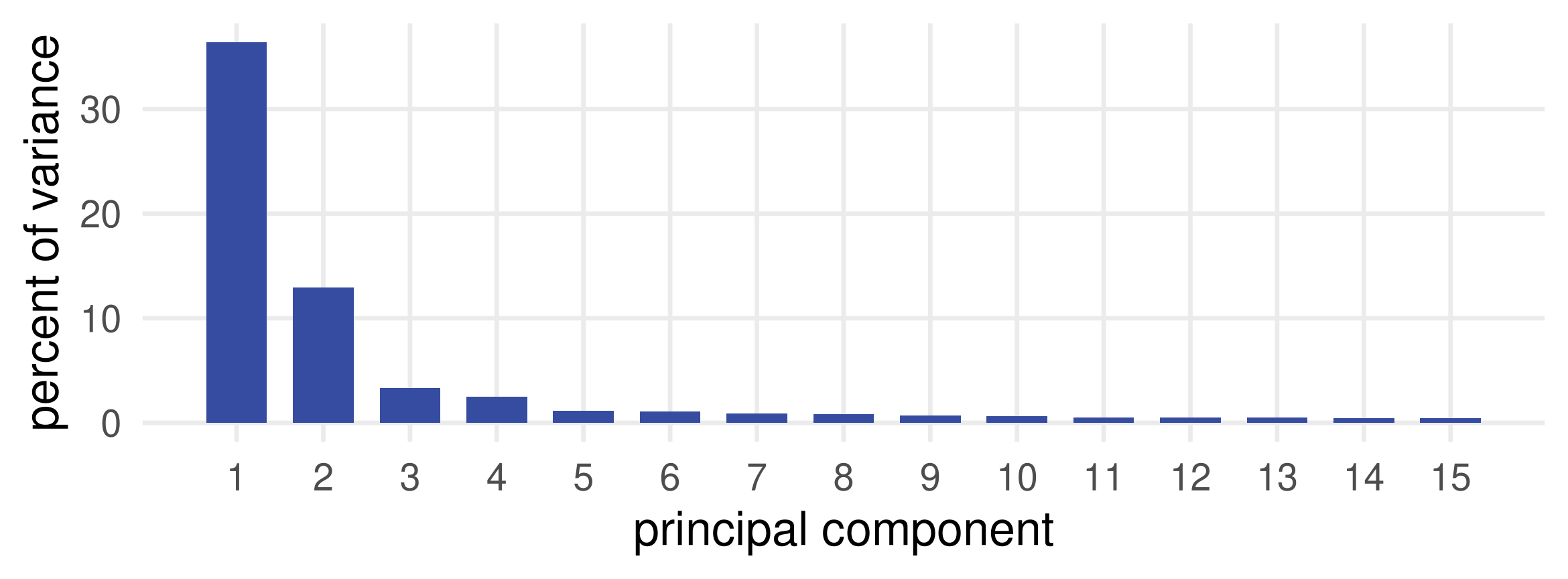

• One component carries 36 percent of the variance of 1,647 votes, a second 13 percent, and nothing else more than 4 percent. This is what a scree plot with a cliff looks like.

Compare the protein scree plot, where the drop was gentle. Here the first two components are a different order of magnitude from the rest.

The first component is ideology

votepc <- predict(pcavote)
round(sort(votepc[, 1])[1:4], 1)                       # most negative

##    BROUN (R GA-10)     FLAKE (R AZ-6) HENSARLIN (R TX-5)   LAMBORN (R CO-5) 
##              -39.4              -38.3              -37.6              -37.4

round(sort(votepc[, 1], decreasing = TRUE)[1:4], 1)    # most positive

##  EDWARDS (D MD-4)    PRICE (D NC-4)   MATSUI (D CA-5) SCHAKOWS (D IL-9) 
##              25.3              25.2              25.1              25.0

table(party = legis$party, PC1_positive = votepc[, 1] > 0)

##      PC1_positive
## party FALSE TRUE
##    D      9  253
##    DR     1    0
##    R    182    0

• The most negative scores are conservative Republicans, the most positive are liberal Democrats; the sign of the score alone classifies 435 of 445 members. The nine Democrats on the negative side are the conservative wing.
• This is the horizontal axis of the opening slide. Political scientists estimate it with purpose-built models (Poole and Rosenthal); PCA gets most of the way in one line.

No label went in. The parties come out because the largest source of variation among 1,647 votes is how often a member votes with one party’s majority. The sign is arbitrary, as always; here negative happens to be right.

The second component: the members at the bottom

round(sort(votepc[, 2])[1:5], 1)

##      SOLIS (D CA-32) GILLIBRAND (D NY-20)      PELOSI (D CA-8)    STUTZMAN (R IN-3) 
##                -88.3                -87.6                -86.5                -85.6 
##       REED (R NY-29) 
##                -85.5

abstain <- rowSums(votes == 0); names(abstain) <- legis$member
sort(abstain, decreasing = TRUE)[1:5]

##      SOLIS (D CA-32) GILLIBRAND (D NY-20)       REED (R NY-29)    STUTZMAN (R IN-3) 
##                 1628                 1619                 1562                 1557 
##      PELOSI (D CA-8) 
##                 1541

cor(votepc[, 2], abstain)

## [1] -0.9748882

• The five lowest scores belong to the five members who missed almost every vote: two who left for the Senate and the cabinet in early 2009, the Speaker, who by custom votes rarely, and two elected in November 2010.
• The second component is attendance: its correlation with the number of abstentions is -0.98.

Solis became Secretary of Labor and Gillibrand a Senator in early 2009; Stutzman and Reed won special elections on 2 November 2010; Speaker Pelosi, by House custom, votes only occasionally. The data do not know any of this; they only see rows of zeros.

Why attendance is a component

load2 <- pcavote$rotation[, 2]
top <- names(sort(abs(load2), decreasing = TRUE))[1:5]
round(load2[top], 3)

## Vote.1146  Vote.658 Vote.1090 Vote.1104 Vote.1149 
##     0.056     0.055     0.053     0.052     0.052

colSums(votes[, top] == 1)         # yeas on the five votes that load most on PC2

## Vote.1146  Vote.658 Vote.1090 Vote.1104 Vote.1149 
##       429       432       423       420       426

• The votes with the largest loadings on PC2 were near-unanimous symbolic resolutions: Vote 1146 is “Supporting the goals and ideals of a Cold War Veterans Day”, 429 yeas, 16 abstentions, no nays.
• PCA centres each column. The mean of such a vote is about 0.96, so a yea is +0.04 after centring and an abstention is -0.96. On a thousand such votes, a member who was absent sits far from everyone else, and that distance is the second-largest source of variance in the data.

Had the data not been centred, the first component would have pointed at the mean vote instead. Centring is what makes the component measure deviation from typical behaviour, and here the most atypical behaviour after partisanship is absence. The appendix returns to centring.

The lesson, and a clustering cross-check

A principal component is the direction of largest variance, whatever that direction means. Ideology was first because members disagree most along party lines; attendance was second because a few members missed everything. The method does not know which one you wanted.

K-means with two groups on the same scaled votes, no labels:

set.seed(0)
table(cluster = kmeans(scale(votes), centers = 2, nstart = 10)$cluster, party = legis$party)

##        party
## cluster   D  DR   R
##       1   8   1 182
##       2 254   0   0

Clustering recovers the parties for 436 of 445 members, eight of the same nine conservative Democrats crossing over. Two unsupervised methods, one latent structure.

The agreement is reassuring but expected: when the first component separates two tight groups, the two cluster centres sit at the two ends of that component.

The macroeconomy in one factor: FRED-MD

FRED-MD (McCracken and Ng 2016) is a monthly panel of 126 US series: output, employment, prices, interest rates, money. Row 1 of the file holds each series’ transformation code (levels, differences, log differences) to make it stationary.

raw <- read.csv("data/2024-07-fredmd.csv", check.names = FALSE)
tcode <- as.numeric(raw[1, -1])                      # transformation code of each series
fred <- raw[-1, ]; fred$sasdate <- as.Date(fred$sasdate, "%m/%d/%Y")
fredx <- as.data.frame(mapply(fredmd_transform, fred[, -1], tcode))   # function in the appendix
fredx$date <- fred$sasdate
fredx <- filter(fredx, date >= as.Date("1960-01-01"), date <= as.Date("2019-12-01"))
keep <- names(fredx)[colSums(is.na(fredx)) == 0 & names(fredx) != "date"]
c(months = nrow(fredx), series = length(keep))

## months series 
##    720    121

pcfred <- prcomp(fredx[, keep], scale = TRUE)
round(100 * summary(pcfred)$importance[2, 1:6], 1)

##  PC1  PC2  PC3  PC4  PC5  PC6 
## 14.9  7.4  7.1  5.6  4.3  3.5

Five series with missing values (consumer sentiment, new orders, the trade-weighted dollar, VIX) are dropped so that the panel is balanced. The sample ends in 2019 to keep the pandemic months, which are outliers in every series, out of the picture. Stock and Watson (2002) call the components “diffusion indexes”.

The business cycle factor

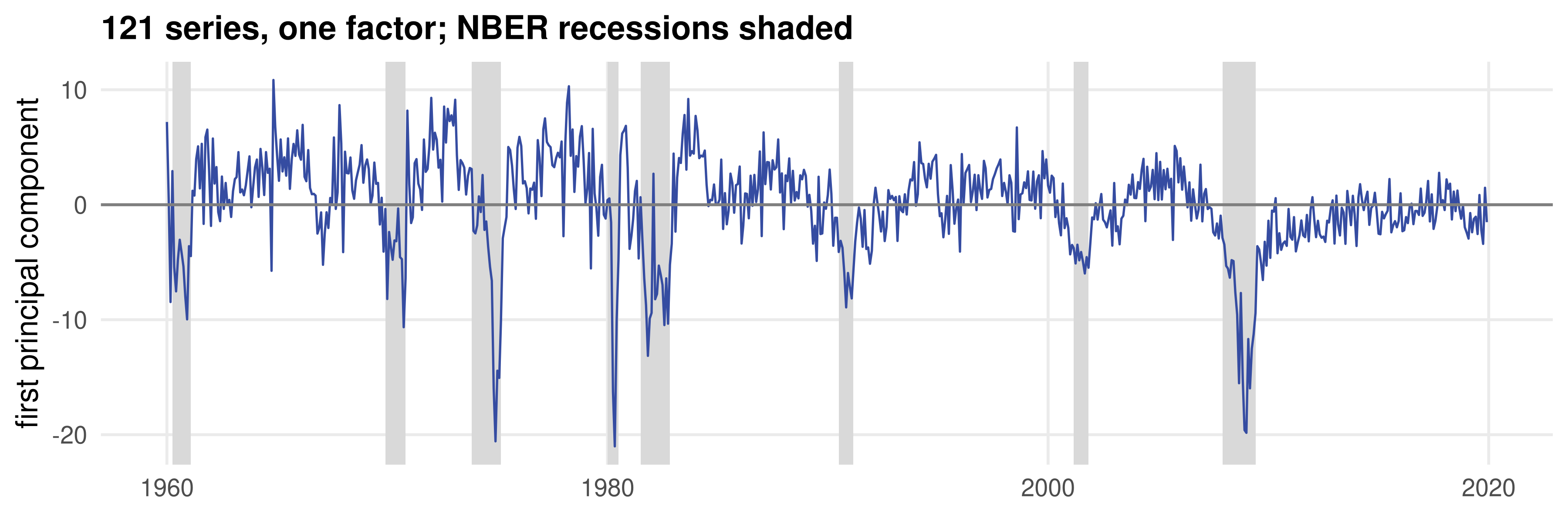
• The first component of 121 series, 15 percent of their variance, falls in every recession and troughs in the deepest ones. Nothing about dates or recessions went in.
• Its loadings are positive on payroll employment and industrial production and negative on the unemployment rate and claims: a real activity factor.

The correlation of the factor with monthly industrial production growth is 0.82. The second component loads on consumer price indexes and on interest rate spreads: a nominal factor. The Chicago Fed’s National Activity Index is built in exactly this way from 85 series.

Reading the macro loadings

phi1 <- sgn * pcfred$rotation[, 1]
round(sort(phi1, decreasing = TRUE)[1:5], 2)     # payrolls, manufacturing output, goods employment

##    PAYEMS IPMANSICS    USGOOD    INDPRO    MANEMP 
##      0.20      0.20      0.20      0.19      0.19

round(sort(phi1)[1:5], 2)                        # unemployment rate, long-term unemployed, claims

##   UNRATE UEMP15OV ISRATIOx  CLAIMSx UEMP27OV 
##    -0.13    -0.10    -0.10    -0.09    -0.08

round(sort(pcfred$rotation[, 2], decreasing = TRUE)[1:4], 2)   # consumer and PCE price indexes

##     CUSR0000SAC DNDGRG3M086SBEA   CUSR0000SA0L2        CPIAUCSL 
##            0.24            0.24            0.24            0.23

• A loading vector is a recipe: the first factor is a weighted sum of 121 standardized series, employment and output positive, unemployment negative.
• The second factor is prices: the consumer price index and its components, the PCE price index. Inflation is the next largest common movement after the cycle.
• A few components summarize a hundred series; section 5 puts them into a regression.

Series names are FRED mnemonics: PAYEMS is nonfarm payrolls, IPMANSICS manufacturing production, USGOOD goods-producing employment, UNRATE the unemployment rate, UEMP15OV the long-term unemployed, CLAIMSx initial claims, CPIAUCSL the consumer price index, PCEPI the PCE price index.

Principal components regression

---

From unsupervised to supervised

• PCA finds the few directions that best explain the variation in X.
• If some Y depends on X through the same latent factors, those directions should predict Y too.
• Principal components regression (PCR): do PCA on the X_i, then regress Y_i on the scores \hat Z_{i1}, \dots, \hat Z_{iK}.

Why it can work when OLS on X does not:

• K regressors instead of d, with K \ll d, so OLS is well-behaved even when d is close to n or above it;
• the scores are uncorrelated and ordered, so adding the (K+1)th does not disturb the first K;
• K is a complexity parameter with an out-of-sample loss, so cross-validation chooses it.

The risk is in the “if”: PCA orders the components by their variance in X, not by their relation to Y. A direction with little variance in X can matter for Y and arrive late in the sequence. The spending example shows this.

The algorithm

1. Do PCA on X_1, \dots, X_n to obtain \hat Z_{i1}, \dots, \hat Z_{iK_{\max}} for some large K_{\max}, for instance K_{\max} = d if d \le n.
2. Apply a supervised method to predict Y_i from the scores:
   • OLS on the first K scores, for each K \le K_{\max}, with cross-validation choosing K. Because the components are nested and uncorrelated, this is one sequence of fits.
   • Or a lasso on the scores, or on the scores together with the original X_i, letting the penalty choose between raw variables and factors.

Neither step is new. Step 1 is section 3; step 2 is lectures 10 and 12. What is new is treating the unsupervised output as an input.

Related methods with the same structure: partial least squares chooses the directions using Y as well, and ridge regression can be read as shrinking along the principal components in proportion to their variance (Hastie, Tibshirani and Friedman, sections 3.4 and 3.5).

Online spending, continued

Lecture 12 predicted a household’s log spending from the share of its browsing at each of 1,000 websites. The lasso reached an out-of-sample R^2 of 0.11; OLS on all 1,000 sites was below zero. Same data, same split.

yspend <- read.csv("data/browser-totalspend.csv")$spend
web <- read.csv("data/browser-domains.csv")
sitenames <- scan("data/browser-sites.txt", what = "character", quiet = TRUE)
web$site <- factor(web$site, levels = 1:length(sitenames), labels = sitenames)
web$id <- factor(web$id, levels = 1:length(unique(web$id)))
visitpercent <- 100 * web$visits / as.vector(tapply(web$visits, web$id, sum))[web$id]
xweb <- sparseMatrix(i = as.numeric(web$id), j = as.numeric(web$site), x = visitpercent,
                     dims = c(nlevels(web$id), nlevels(web$site)),
                     dimnames = list(levels(web$id), levels(web$site)))
ly <- log(yspend)
set.seed(0); n <- length(ly)
test <- sample.int(n, size = round(0.2 * n)); train <- setdiff(1:n, test)   # 2,000 held out
dim(xweb)

## [1] 10000  1000

The data preparation is copied from lecture 12 so that the hold-out set is the same 2,000 households. prcomp() needs a dense matrix; 10,000 by 1,000 is 80 MB, which is fine.

Does browsing have a few dimensions?

pcweb <- prcomp(as.matrix(xweb), scale = TRUE)   # about 15 seconds
Zweb <- predict(pcweb)
round(100 * summary(pcweb)$importance[3, c(1, 10, 50, 100, 200)], 1)   # cumulative percent

##   PC1  PC10  PC50 PC100 PC200 
##   1.7   8.4  21.4  32.0  47.3

round(drop(cor(Zweb[train, 1:8], ly[train])), 2)                       # each score against log spending

##   PC1   PC2   PC3   PC4   PC5   PC6   PC7   PC8 
##  0.11 -0.02 -0.01 -0.09  0.06  0.05 -0.01 -0.09

• No: the first component explains under 2 percent of the variance and a hundred components under a third. Browsing shares are spread across many weak patterns, nothing like the one-factor Congress.
• The scores’ correlations with spending are small and not ordered: the first component is the most related to spending, the fourth is next, the second and third are useless. PCA did not look at Y.

Scaling each site’s column matters again: without it, the components reproduce the few giant sites (google, yahoo, msn) and carry nothing about spending; the comparison slide reports that case.

Cross-validating K

Kgrid <- c(1:60, seq(70, 200, 10))
set.seed(0); fold <- sample(rep(1:10, length.out = length(train)))
cv_mse <- sapply(Kgrid, function(k) {
  err <- 0
  for (i in 1:10) {
    tr <- train[fold != i]; te <- train[fold == i]
    b <- lm.fit(cbind(1, Zweb[tr, 1:k]), ly[tr])$coefficients
    err <- err + sum((ly[te] - cbind(1, Zweb[te, 1:k]) %*% b)^2)
  }
  err / length(train)
})
K_best <- Kgrid[which.min(cv_mse)]
c(K_best = K_best, cv_mse = min(cv_mse), null_mse = var(ly[train]))

##    K_best    cv_mse  null_mse 
## 48.000000  2.547223  2.787185

Ten folds within the 8,000 training households, as in lecture 12; the held-out 2,000 are not touched until the next slide. lm.fit() is lm() without the formula overhead, which matters for 74 values of K times 10 folds.

The cross-validation curve

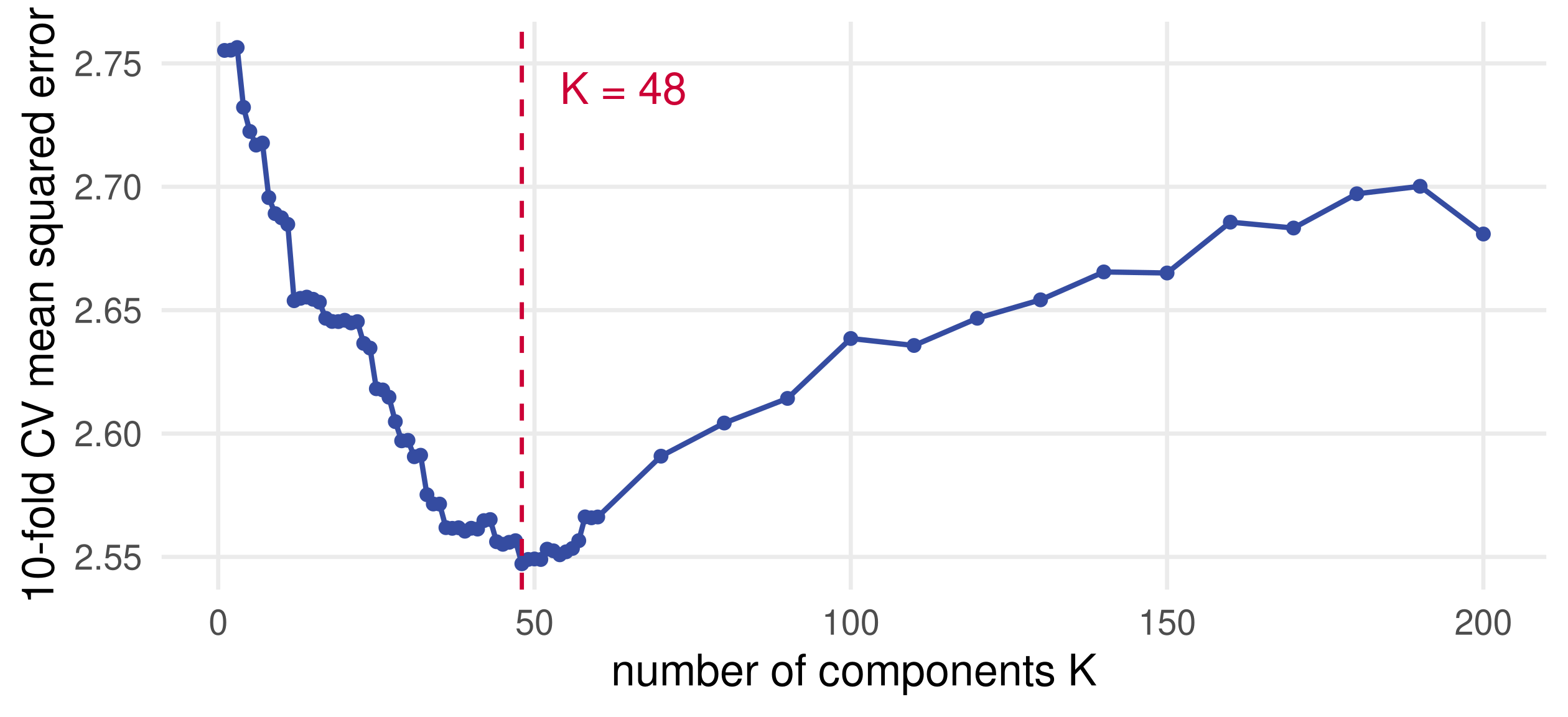
• The familiar U: too few components underfit, too many let OLS chase noise. The minimum is at 48 components, against a null mean squared error of 2.79.
• The decline is slow because the predictive directions arrive in no particular order; the curve has to wait for them.

Compare lecture 12’s cv.glmnet() curve over lambda. Same logic, different complexity parameter: there the number of nonzero coefficients, here the number of components.

PCR against the lasso, out of sample

b_pcr <- lm.fit(cbind(1, Zweb[train, 1:K_best]), ly[train])$coefficients
set.seed(0); cv_lasso <- cv.glmnet(xweb[train, ], ly[train])                         # lecture 12
set.seed(0); cv_both <- cv.glmnet(cbind(xweb, Zweb[, 1:100])[train, ], ly[train])    # sites and scores
b_both <- coef(cv_both, s = "lambda.min")[-1]
data.frame(model = c("PCR, K chosen by CV", "Lasso on 1,000 sites", "Lasso on sites and 100 scores"),
       inputs_used = c(K_best, sum(coef(cv_lasso, s = "lambda.min")[-1] != 0),
                       paste(sum(b_both[1:1000] != 0), "sites +", sum(b_both[1001:1100] != 0), "scores")),
       out_of_sample_r2 = round(c(
         r2(ly[test], cbind(1, Zweb[test, 1:K_best]) %*% b_pcr, mean(ly[train])),
         r2(ly[test], predict(cv_lasso, xweb[test, ], s = "lambda.min"), mean(ly[train])),
         r2(ly[test], predict(cv_both, cbind(xweb, Zweb[, 1:100])[test, ], s = "lambda.min"), mean(ly[train]))), 3))

##                           model           inputs_used out_of_sample_r2
## 1           PCR, K chosen by CV                    48            0.100
## 2          Lasso on 1,000 sites                   228            0.107
## 3 Lasso on sites and 100 scores 163 sites + 20 scores            0.111

• PCR with 48 components matches the lasso with 228 sites on the held-out households: two different models, the same ten percent of variance explained.
• Offered both, the lasso keeps 163 sites and 20 scores: factors and raw variables are complements. With unscaled site shares, no number of components gets the hold-out R^2 above 0.02.

The unscaled result is from the same code with scale = FALSE in prcomp(); it is not shown to save fifteen seconds of rendering. The components then follow the giant sites, which say nothing about spending. The lesson is the one from K-means: the scale of X is a modelling choice that PCA cannot make for you.

What the spending example shows

• PCA ignores Y. Components are ordered by their variance in X. The predictive ones were the 1st, the 4th, the 8th, and so on, so PCR needed 48 components to collect them.
• Scale decides the components. Unscaled, PCA described a handful of giant sites and PCR failed; scaled, it described browsing patterns and PCR worked.
• K is now a tuning parameter with an out-of-sample loss, and cross-validation chooses it exactly as it chose \lambda for the lasso and the tree size last week.
• Unsupervised output is supervised input. The forest and the lasso of earlier lectures accept scores as regressors; the lasso can even choose between scores and raw variables.

The honest summary: on these data PCR is as good as the lasso and no better. Its advantage shows when the regressors are strongly collinear and a few factors really do drive both X and Y, as with the macro panel, where a factor-augmented regression is the standard forecasting tool.

Checkpoint: PCR

1. Lecture 12 found OLS on all 1,000 sites had an out-of-sample R^2 below zero. Why does OLS on 48 principal component scores not suffer the same fate?
2. Why can the cross-validation curve over K be computed with a single ordering of regressors, when the lasso needed a whole path of penalties?
3. A colleague proposes choosing K from the scree plot of X and then regressing Y on those K scores. What could go wrong?

Answers: 48 regressors against 8,000 observations is a small model, and the scores are uncorrelated, so the coefficients are estimated precisely; 1,000 correlated regressors spread the same information over a thousand noisy coefficients. The components are nested and ordered, so the fit for K is the fit for K minus 1 plus one regressor; the lasso’s active set changes with lambda. The scree plot ranks components by their variance in X, not their relation to Y; on the browsing data the components that predict spending are scattered through the list, so a small K from the scree plot would miss them.

Unsupervised learning in one page

No Y, no out-of-sample check. The goal is to describe X with fewer numbers; the discipline against invented structure has to come from replication, scaling and interpretation.

Two latent-variable models, two methods. A mixture model with a hidden type gives K-means: alternate centres and nearest-centre assignments until nothing moves. A linear factor model with hidden continuous factors gives PCA: the K-dimensional plane closest to the cloud, computed by one singular value decomposition.

K-means finds a local minimum of the within-cluster sum of squares. Use many starts, scale the columns, and treat K as a question of interpretation.

Principal components are nested, uncorrelated and ordered by variance. Loadings say what a component is; scores say where each observation sits; the scree plot and variance shares say how many matter. The largest direction is whatever varies most, be it ideology, attendance or the business cycle.

Factors make regressors. Principal components regression turns the scores into inputs for OLS or the lasso and gives K an out-of-sample criterion again. PCA does not look at Y, so the useful components may come late.

Reading and data sources

• James, Witten, Hastie and Tibshirani, An Introduction to Statistical Learning, chapter 12: PCA and clustering; section 6.3.1 for principal components regression.
• Hastie, Tibshirani and Friedman, The Elements of Statistical Learning, sections 14.3 (clustering, including the Gaussian mixture limit) and 14.5 (PCA).
• Taddy, Business Data Science (2019), chapter 7: the protein and roll-call data.
• Hartigan and Wong (1979), the K-means algorithm behind kmeans(); Lloyd (1982), the basic iteration.
• Jolliffe and Cadima (2016), a review of PCA.
• Poole and Rosenthal (1985), spatial models of roll-call voting.
• McCracken and Ng (2016), the FRED-MD database; Stock and Watson (2002), forecasting with principal components of many predictors; Bai and Ng (2002), choosing the number of factors.

Additional derivations and code

---

Optional material for reference and practice

Why K-means converges

Write the objective with both arguments, W(C, \mu) = \sum_{i=1}^n \lVert X_i - \mu_{C_i} \rVert^2.

• For fixed memberships C, W is a sum over clusters of \sum_{i \in C_k} \lVert X_i - \mu_k \rVert^2, which is minimized by the cluster mean. Step 2 cannot increase W.
• For fixed centres \mu, each term \lVert X_i - \mu_{C_i} \rVert^2 is minimized by sending i to its nearest centre. Step 3 cannot increase W.
• W is bounded below and there are finitely many partitions, so the sequence stops after finitely many steps, at a partition no single step improves: a local minimum.

Centres can be eliminated: for a cluster of size n_k,

\sum_{i \in C_k} \lVert X_i - \bar X_k \rVert^2 = \frac{1}{2 n_k} \sum_{i \in C_k} \sum_{i' \in C_k} \lVert X_i - X_{i'} \rVert^2,

so K-means also minimizes the within-cluster pairwise squared distances, each cluster’s sum scaled by its size. Hastie, Tibshirani and Friedman (section 14.3) introduce clustering through this pairwise form.

K-means as a limit of the Gaussian mixture

In a Gaussian mixture with common variance \sigma^2, the EM algorithm alternates two steps:

• E step. The posterior probability that observation i came from component k, r_{ik} = \frac{\pi_k \exp\{-\lVert X_i - \mu_k \rVert^2 / 2\sigma^2\}}{\sum_{l} \pi_l \exp\{-\lVert X_i - \mu_l \rVert^2 / 2\sigma^2\}}.
• M step. \mu_k becomes the r_{ik}-weighted average of the X_i, and \pi_k the average of r_{ik}.

As \sigma^2 \to 0, the exponential with the smallest distance dominates every other, so r_{ik} \to 1 for the nearest centre and 0 otherwise. The E step becomes step 3 of K-means, the M step becomes step 2, and the weights \pi_k drop out. K-means is EM with hard assignments; EM with finite \sigma^2 is “soft K-means” (Hastie, Tibshirani and Friedman, section 14.3.7).

The first component maximizes variance

Let S be the d \times d sample covariance matrix of the centred data. The variance of the projection X_i'\varphi is \varphi' S \varphi. The first loading solves

\max_{\varphi}\; \varphi' S \varphi \quad \text{subject to} \quad \varphi'\varphi = 1.

The Lagrangian \varphi' S \varphi - \lambda(\varphi'\varphi - 1) has first-order condition S\varphi = \lambda\varphi: \varphi is an eigenvector of S and the variance it achieves is \varphi' S \varphi = \lambda. So \hat\varphi_1 is the eigenvector with the largest eigenvalue \lambda_1, and \hat{\operatorname{Var}}(\hat Z_{\cdot 1}) = \lambda_1.

• Adding the constraint \varphi'\hat\varphi_1 = 0 gives the second eigenvector, and so on. The eigenvalues sum to \operatorname{tr}(S), the total variance, which is d after scaling: that is the “proportion of variance explained”.
• Minimum reconstruction error gives the same answer: for a unit vector \varphi, \lVert X_i \rVert^2 = (X_i'\varphi)^2 + \lVert X_i - (X_i'\varphi)\varphi \rVert^2, so minimizing the summed residuals is maximizing the summed projections.
• With X = UDV', S = V (D'D/(n-1)) V', so the eigenvectors are the columns of V and \lambda_k = d_k^2/(n-1): the singular value decomposition of section 3 and the eigenvalues here are the same computation.

Reading prcomp() through the SVD

Every claim on the SVD slide, checked on the protein data:

sv <- svd(xfood)                                                # xfood is centred and scaled
all.equal(sv$d / sqrt(nrow(xfood) - 1), pcfood$sdev)            # sdev = d_k / sqrt(n - 1)

## [1] TRUE

all.equal(abs(unname(sv$v[, 1:5])), abs(unname(pcfood$rotation)))   # loadings = columns of V, up to sign

## [1] TRUE

all.equal(abs(unname(xfood %*% sv$v[, 1:5])), abs(unname(food_factors)))   # scores = X V = U D

## [1] TRUE

round(cor(food_factors), 2)[1:3, 1:3]                           # scores are uncorrelated

##     PC1 PC2 PC3
## PC1   1   0   0
## PC2   0   1   0
## PC3   0   0   1

round(sum(pcfood$sdev^2), 6)                                    # variances sum to d = 9

## [1] 9

abs() handles the arbitrary sign of each component. pcfood$x is the same matrix as predict(pcfood).

Why centring matters

PCA minimizes the sum of squared distances from the centred data to a K-dimensional subspace through the origin. Without centring, the subspace must pass through the origin of the raw data rather than through the point cloud, and the first component mostly points from the origin towards the mean \bar X.

• For the roll-call votes, the raw mean of a near-unanimous resolution is 0.96. Uncentred, the first component would be “how much a member votes yea on everything”, which is attendance mixed with the number of resolutions, not ideology.
• Centred, a yea on such a vote is +0.04 and an abstention -0.96: the column contributes almost nothing unless a member was absent, and absence becomes a component of its own only because the five absentees were absent on hundreds of such columns at once.
• prcomp() centres by default (center = TRUE); scale = TRUE is the choice you must make.

The FRED-MD transformation codes

Each series in FRED-MD carries a code for the transformation that makes it stationary (McCracken and Ng 2016, Appendix). The function used on the FRED-MD slide:

fredmd_transform <- function(x, code) {
  switch(as.character(code),
    "1" = x,                                           # level
    "2" = c(NA, diff(x)),                              # first difference
    "3" = c(NA, NA, diff(x, differences = 2)),         # second difference
    "4" = log(x),                                      # log
    "5" = c(NA, diff(log(x))),                         # log difference: a growth rate
    "6" = c(NA, NA, diff(log(x), differences = 2)),    # change in the growth rate
    "7" = c(NA, NA, diff(x[-1] / x[-length(x)] - 1)))  # change in the percentage change
}

mapply(fredmd_transform, fred[, -1], tcode) applies each series’ own code. Codes 5 and 6 dominate: 52 series are growth rates and 33 are changes in growth rates (prices).

Install the required packages

Run once in your R environment if needed:

install.packages(c("tidyverse", "patchwork", "Matrix", "glmnet"))

Data files, all read from lectures/data/:

• protein.csv, the 25 countries and nine food groups;
• rollcall-votes.csv and rollcall-members.csv, the 111th House;
• 2024-07-fredmd.csv, the FRED-MD panel through June 2024, used through December 2019;
• browser-totalspend.csv, browser-domains.csv and browser-sites.txt, the online spending panel of lecture 12.

kmeans(), prcomp() and svd() are in base R.

Return to the question

A computer found the parties: the first principal component of 1,647 votes is an ideology score that classifies 435 of 445 members by its sign, and two-cluster K-means recovers the parties for 436. The members trailing off the bottom were the second component, attendance, because PCA reports the largest variation it finds, whatever it means.

Return to the main takeaway