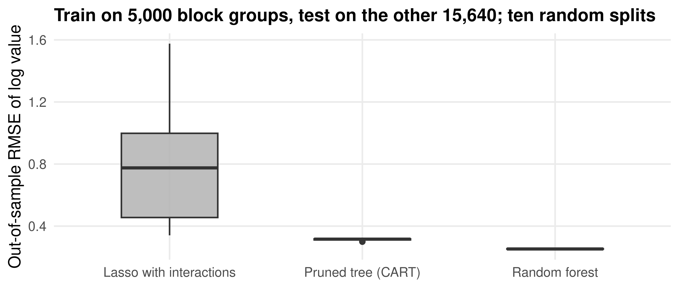
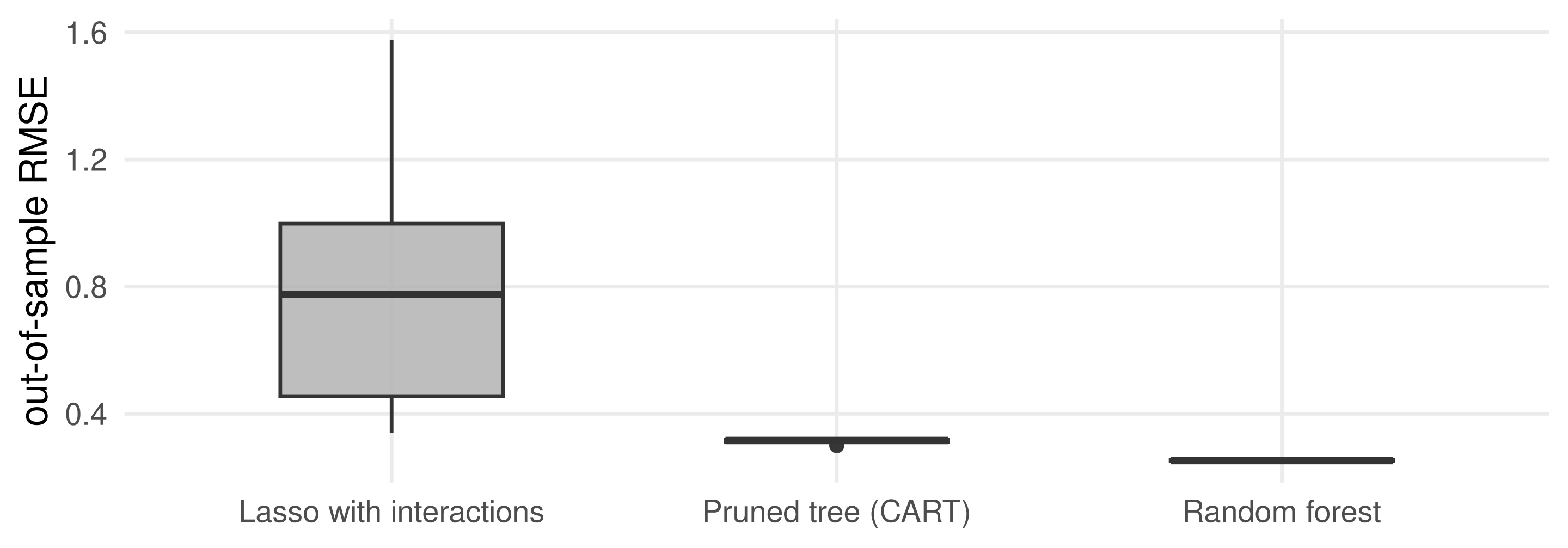
The random forest predicts best, with no tuning parameter chosen by cross-validation.
A single pruned tree comes second. The lasso, with every covariate interacted with longitude and latitude, is erratic: one block group with 1,243 persons per household wrecks it whenever it lands in the test set.
Today’s route
From bins to trees: the binned sample mean, its two problems, and the tree as a data-chosen set of bins.
Growing a tree: a deviance to minimize, the greedy split, and tree() on motorcycle crashes and TV shows.
Pruning: why stopping rules fail, weakest-link pruning, cost-complexity and cross-validation.
Random forests: bagging, random covariate subsets, variable importance, and the California housing contest.
library(MASS) # the mcycle data; load before tidyverse so dplyr::select winslibrary(tidyverse)library(tree) # tree(), prune.tree(), cv.tree()library(ranger) # fast random forestslibrary(glmnet) # the lasso, for the comparison at the end
File
Role
MASS::mcycle
Helmet acceleration after a simulated motorcycle crash, 133 readings
40 TV shows: genre, ratings, engagement and audience shares
data/prostate.csv
97 prostate cancer patients
data/CAhousing.csv
20,640 California census block groups
From bins to trees
A tree is a binned sample mean whose bins are chosen by the data
Recall the binned sample mean
In lecture 11 we predicted Y from a scalar X by
cutting the range of X into bins at sample quantiles, and
predicting Y_{n+1} by the average of the Y_i whose X_i fall in the same bin as X_{n+1}.
The number of bins was the complexity parameter, and cross-validation chose it.
Two things were unsatisfying.
Bins of equal count everywhere. If \mathbf{E}[Y \mid X = x] is flat in some regions and wiggly in others, the bins should be wide where it is flat and narrow where it is wiggly.
Only one covariate. With d covariates and c cutpoints on each, cutting the sample by every variable gives (c+1)^d bins.
The curse of dimensionality
With c = 4 cutpoints per covariate, the grid of bins grows as 5^d:
Covariates d
Bins 5^d
Observations per bin when n = 20{,}640
1
5
4,128
2
25
826
5
3,125
7
9
1,953,125
0.01
Most bins are empty long before d reaches ten. We need bins that are adaptive: narrow only along the covariates and in the regions where Y actually changes, and wide elsewhere.
The lasso solved an analogous problem for linear models by selecting covariates. A regression tree is a way of selecting bins.
A decision tree
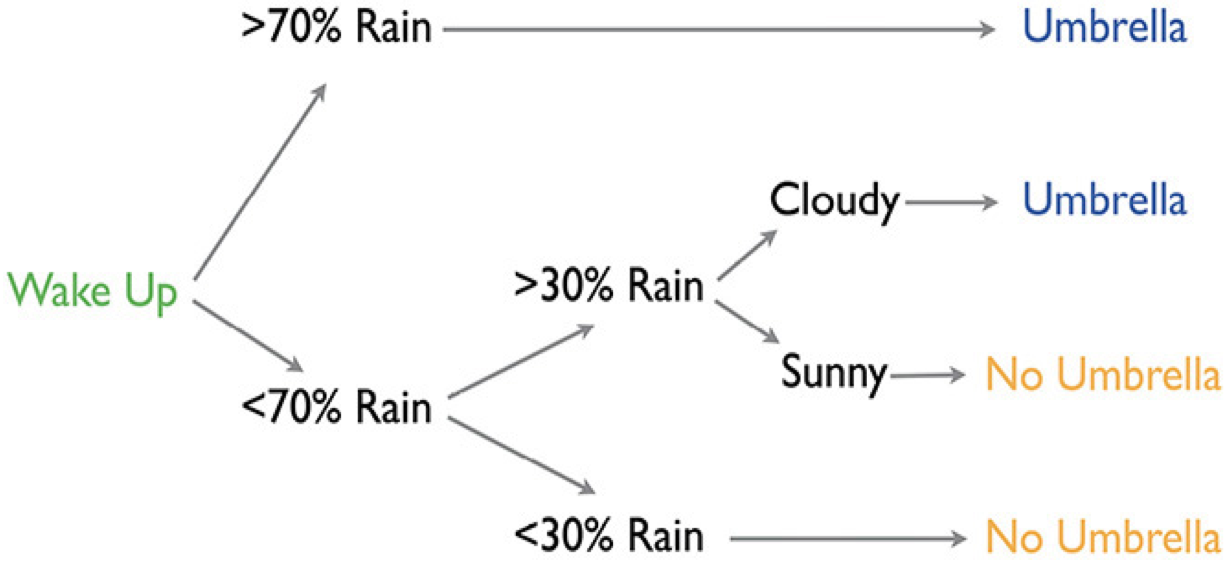
A decision tree is a nested sequence of if-else statements that takes an input and returns a conclusion. Here the input is the weather and the conclusion is whether to carry an umbrella.
The boxes are nodes with a parent and child structure. The nodes at the end, leaves, hold the conclusions.
A diagram of this kind is a dendrogram.
A regression tree
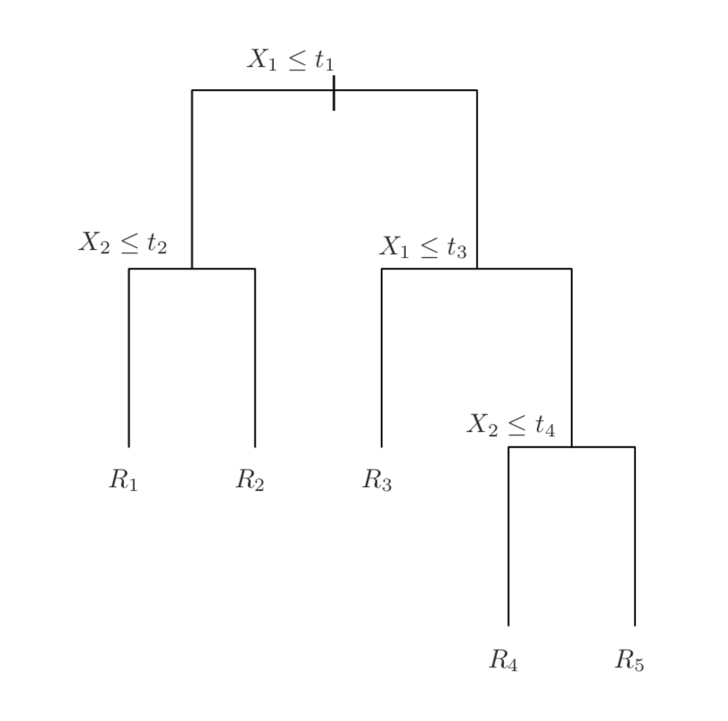
Each internal node is a threshold on one covariate: an observation goes left if X_{i,1} \le t_1 and right otherwise.
Each leaf is a rectangle R_m of the covariate space. X_i lands in R_1 when X_{i,1} \le t_1 and X_{i,2} \le t_2.
What a tree predicts
Send the n observations down the tree. In each leaf, output a prediction from the observations that landed there:
Y real-valued: the leaf mean, \hat{\mathbf{E}}[Y \mid X_1 \le t_1, X_2 \le t_2] in R_1.
Y categorical: the share of each category, \hat{\mathbf{P}}(Y = m \mid X_1 \le t_1, X_2 \le t_2) for every class m.
A new X_{n+1} is dropped down the same tree; its leaf gives the prediction.
A regression tree is the binned sample mean with the bins given by the leaves. The tree decides which covariate to cut, where, and how finely.
The same construction handles classification, so the family is called CART, classification and regression trees. We say “regression tree” for both.
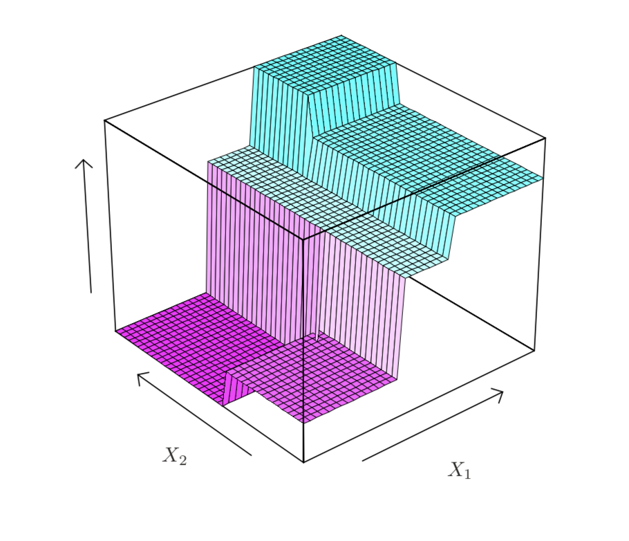
The fitted function is a step function
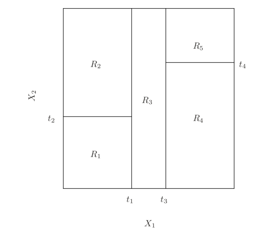
Left: \hat f(x) = \sum_m \hat c_m \, \mathbf{1}\{x \in R_m\} is constant on each leaf and jumps at the thresholds.
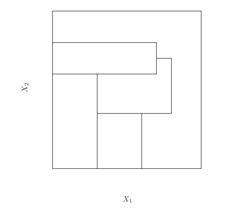
The partition is a recursive binary partition: each split cuts one existing rectangle in two. Right: a partition no tree can produce, because the first cut would have to run through a region.
Checkpoint: bins and trees
A tree splits first on X_1 at 3, then splits the left child on X_2 at 10. How many leaves are there, and which rectangle does (X_1, X_2) = (2, 12) fall in?
Why does cutting every covariate at its quartiles fail with nine covariates and 20,000 observations?
In what sense is a regression tree “adaptive” where the quantile bins of lecture 11 were not?
Growing a tree
A deviance to minimize and a greedy search
A deviance to minimize
Which tree? As with every estimator this semester, choose the one that minimizes a deviance, a loss function summed over the sample.
Y real-valued, sum of squares: \sum_{i=1}^n \big(Y_i - \hat{\mathbf{E}}[Y \mid X_i]\big)^2, \qquad \text{OLS used } X_i'\hat\beta \text{ in place of } \hat{\mathbf{E}}[Y \mid X_i].
Y categorical with K classes, multinomial deviance: -2\sum_{i=1}^n \sum_{k=1}^K \mathbf{1}\{Y_i = k\} \log \hat{\mathbf{P}}(Y_i = k \mid X_i).
Most software offers the Gini impurity instead, \sum_i \sum_k \hat p_k(X_i)\,(1 - \hat p_k(X_i)), which estimates the variance of \mathbf{1}\{Y_i = k\} in each leaf. The two rarely disagree.
The search is greedy
Minimizing the deviance over all trees is infeasible: the number of trees grows exponentially with the number of splits.
Instead, recursive binary splitting builds the tree one split at a time. For the first split, consider every covariate j and every observed value s of X_{ij}:
Pick the (j, s) with the smallest deviance. Then repeat inside each child, using only its observations, and keep going.
The first split by hand: motorcycle crashes
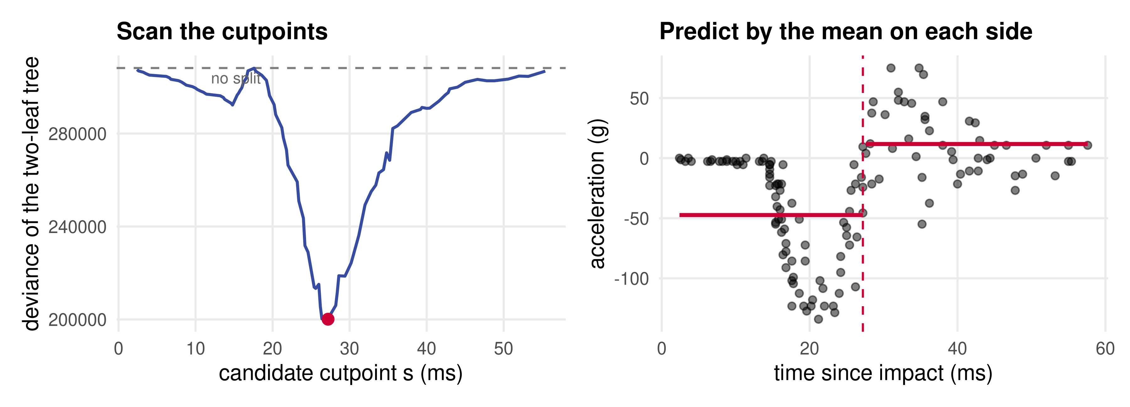
mcycle records helmet acceleration (in g) against time (ms) after a simulated impact. Scan every candidate cutpoint s on times and record the deviance of the two-leaf tree.
split_deviance <-function(s) { left <- mcycle$accel[mcycle$times <= s] right <- mcycle$accel[mcycle$times > s]sum((left -mean(left))^2) +sum((right -mean(right))^2)}cutpoints <-head(sort(unique(mcycle$times)), -1) # every observed time but the lastdev_path <-tibble(s = cutpoints, deviance =sapply(cutpoints, split_deviance))dev_path |>slice_min(deviance, n =1)
## # A tibble: 1 × 2
##       s deviance
##   <dbl>    <dbl>
## 1  27.2  200123.
sum((mcycle$accel -mean(mcycle$accel))^2) # deviance with no split
## [1] 308222.7
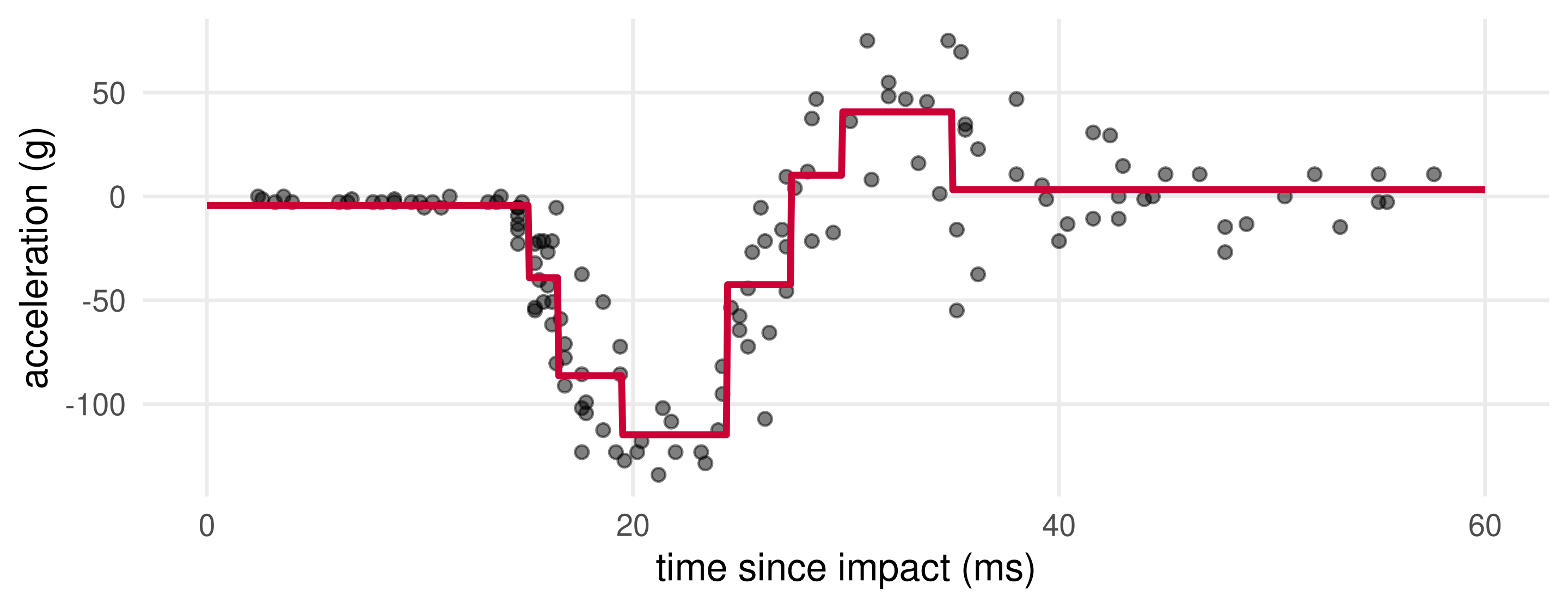
The best single cut is between 27.2 and 27.6 ms and removes a third of the deviance.
The first split, pictured
Both halves are still far from flat. Recursive binary splitting now repeats the scan inside each half.
The CART algorithm and its stopping rules
Find the split (j, s) that minimizes the deviance.
Split the node into left and right children and route the observations.
Repeat steps 1 and 2 in each child.
Stop splitting a node when it is too small or when no split helps enough. That node is a leaf.
In tree() the stopping rules are
Argument
Rule
Default
mincut
each child must contain at least this many observations
5
minsize
a node smaller than this is not split
10
mindev
a split must cut the deviance by at least mindev times the root deviance
0.01
tree() on the motorcycle data
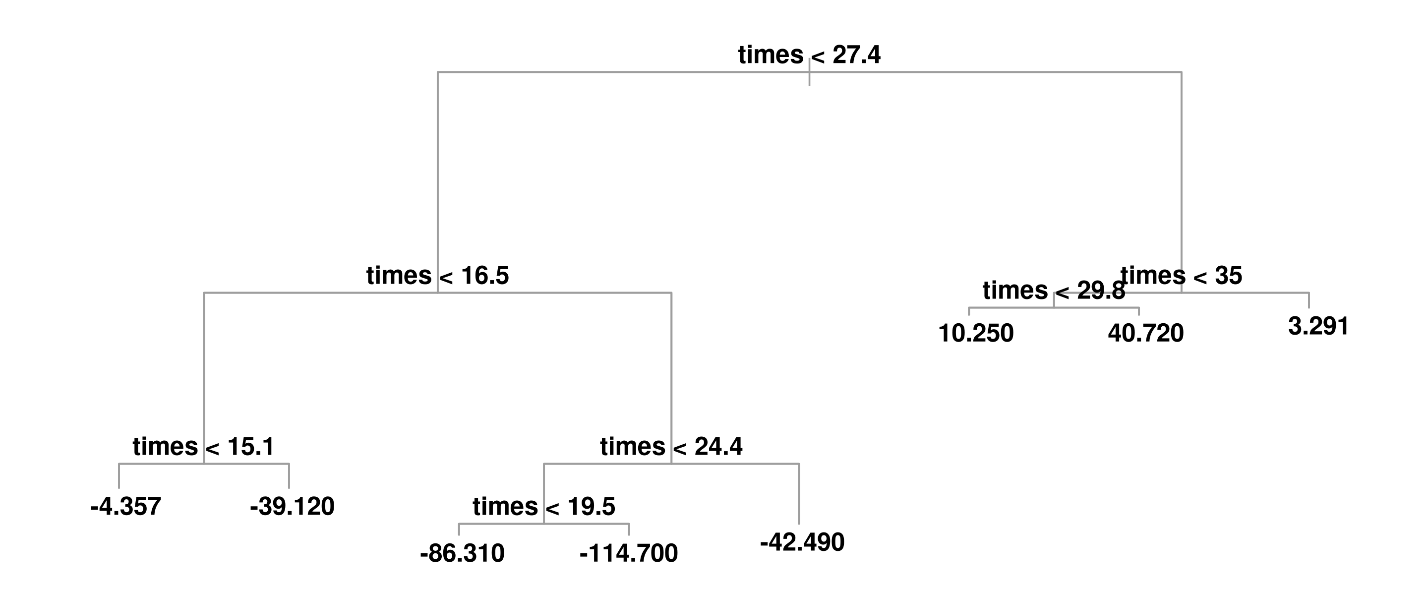
The syntax is that of lm() and glm(). plot() draws the dendrogram and text() labels it.
collision <-tree(accel ~ times, data = mcycle)par(mar =c(1, 2, 1.5, 2), xpd =NA) # room for the labels at the edgesplot(collision, col =8); text(collision, cex =0.85, font =2)
Branch length is proportional to the deviance removed by the split, so the first cut at 27.4 ms is the long one.
Reading the printed tree
collision
## node), split, n, deviance, yval
##       * denotes terminal node
##
##  1) root 133 308200.0  -25.550
##    2) times < 27.4 84 160500.0  -47.320
##      4) times < 16.5 43  18020.0  -16.480
##        8) times < 15.1 28    724.1   -4.357 *
##        9) times > 15.1 15   5494.0  -39.120 *
##      5) times > 16.5 41  58660.0  -79.660
##       10) times < 24.4 27  17040.0  -98.940
##         20) times < 19.5 15   9045.0  -86.310 *
##         21) times > 19.5 12   2616.0 -114.700 *
##       11) times > 24.4 14  12240.0  -42.490 *
##    3) times > 27.4 49  39670.0   11.780
##      6) times < 35 16  13300.0   29.290
##       12) times < 29.8 6   3900.0   10.250 *
##       13) times > 29.8 10   5919.0   40.720 *
##      7) times > 35 33  19080.0    3.291 *
##                   TERRITORY.EAST.CENTRAL TERRITORY.NORTHEAST COUNTY.SIZE.A COUNTY.SIZE.B
## Living with Ed                         6                  19            49            31
## Monarch Cove                          10                  14            35            32
## Top Chef                               8                  24            48            31
## Iron Chef America                     13                  25            47            30
##                   WIRED.CABLE.W.O.PAY DBS.OWNER
## Living with Ed                     44        20
## Monarch Cove                       40        29
## Top Chef                           34        23
## Iron Chef America                  30        26
Each row of demos is a show and each column is the percentage of its audience in a demographic cell: region, county size, cable subscription, household size, and so on. We will predict the show’s genre.
A classification tree
Make the outcome a factor, so that tree() fits class shares rather than a mean. With 40 shows we allow leaves of a single observation.
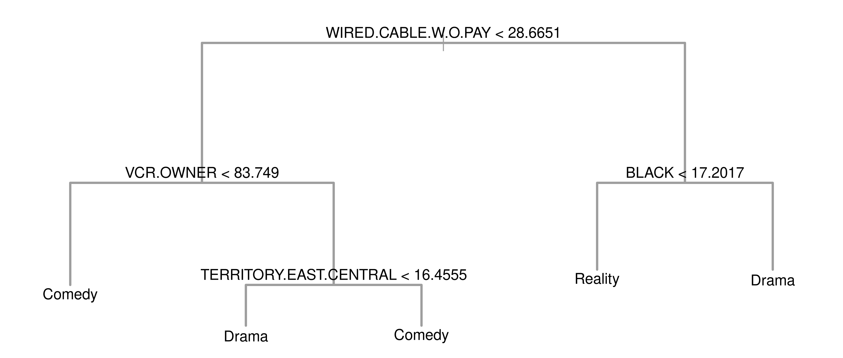
Leaves are labelled with the most likely genre; text(genretree, label = "yprob") prints the three class shares instead. Basic-cable viewers watch reality shows, VCR owners watch drama.
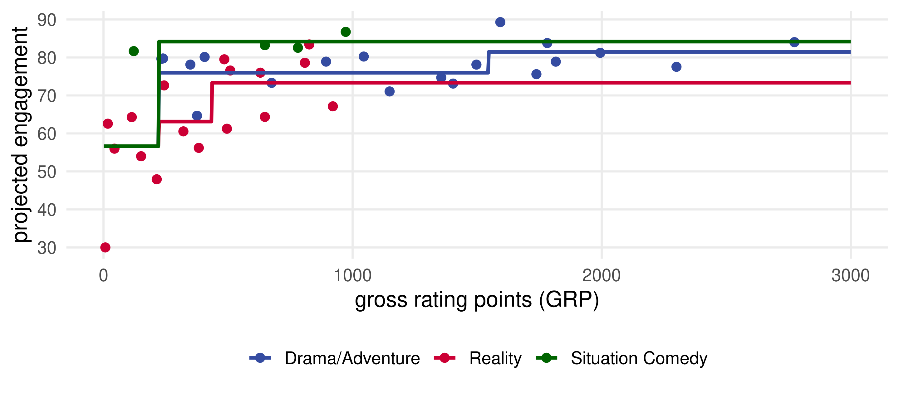
The first split separates the seven low-rated shows; above that, each genre gets its own concave-looking step function.
Checkpoint: growing a tree
In the motorcycle scan, why is the deviance curve flat near the two ends of the time axis?
A node has 12 observations and mincut = 5. Which cutpoints are admissible?
With mindev = 0.01 and a root deviance of 308,000, a node with deviance 19,000 has a best split that removes 950. Is it split?
Pruning
Grow a big tree, then cut it back
Trees overfit
With mincut = 1 and mindev = 0, recursive splitting runs until every leaf holds one observation: the in-sample deviance is zero and the predictor is the nearest-neighbour step function, maximally overfit.
The obvious remedy is to treat mincut and mindev as complexity parameters and cross-validate them. Two things go wrong.
mincut alone forces leaves of similar size everywhere, which is the equal-count binning we wanted to escape.
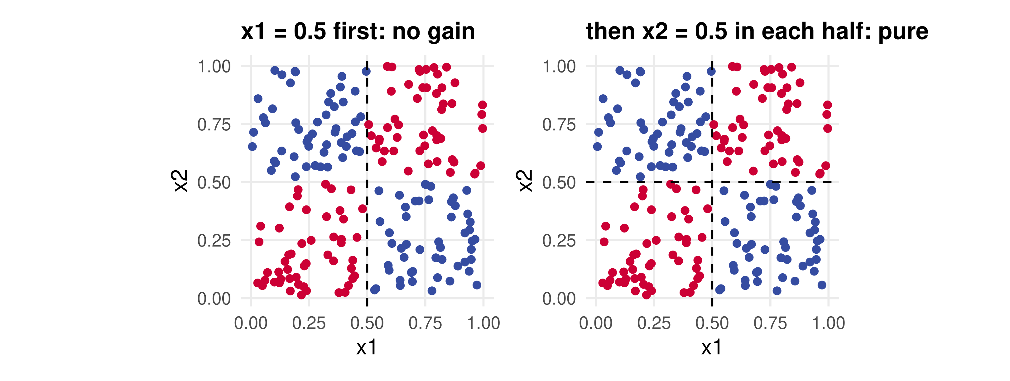
mindev stops when the best next split helps little. But the greedy algorithm lacks foresight: a split that is nearly useless on its own can be the one that makes the next split decisive.
No single split helps, two splits are perfect
tree(y ~ x1 + x2, data = flag, mindev =0.05) # demand a 5% improvement: nothing is ever split
Rather than stop early, overgrow the tree (mindev = 0, small mincut) and then prune it back:
remove the split whose removal increases the deviance the least, turning that node into a leaf;
repeat, producing a nested sequence of subtrees with fewer and fewer leaves.
Pruning does not suffer from the lack of foresight. Breiman, Friedman, Olshen and Stone (1984) show that the sequence contains, for each size, the subtree with the smallest deviance among all subtrees of that size.
The sequence is a set of candidate models indexed by the number of leaves, so cross-validation can choose among them, as it chose the number of bins and the penalty \lambda.
Pruning the genre tree
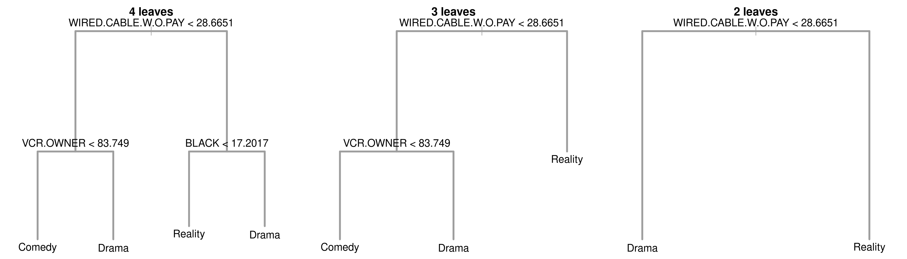
prune.tree(tree, best = m) returns the subtree with m leaves. The genre tree has five, so the sequence runs 5, 4, 3, 2, 1.
par(mfrow =c(1, 3), mar =c(1, 2.5, 2, 2.5), xpd =NA)for (m in4:2) { sub <-prune.tree(genretree, best = m)plot(sub, col =8, lwd =2); text(sub, cex =1.1); title(paste(m, "leaves"), cex.main =1.2)}
The first snip removes TERRITORY.EAST.CENTRAL < 16.4555, a split that separated one comedy from sixteen dramas.
The pruning sequence as a path
Called without best, prune.tree() returns the whole sequence: sizes, in-sample deviances and the threshold k at which each subtree becomes optimal.
genre_path <-prune.tree(genretree)data.frame(size = genre_path$size, deviance =round(genre_path$dev, 2), k =round(genre_path$k, 2))
Each k is the deviance increase per leaf removed by the next snip: snipping node 5 costs 7.61 for one leaf, snipping node 3 costs 16.22, and so on. Larger k means a smaller tree.
Cost-complexity pruning and cross-validation
Penalize the number of leaves, as the lasso penalized the coefficients. For \lambda \ge 0, among subtrees T of the big tree T_0 minimize
\sum_{i=1}^n \big(Y_i - \hat{\mathbf{E}}_T[Y \mid X_i]\big)^2 + \lambda \cdot |T|, \qquad |T| = \text{number of leaves of } T.
The minimizer for each \lambda is a member of the weakest-link sequence, and the k values are the \lambda’s at which the solution changes.
Choosing \lambda by K-fold cross-validation (James et al., Algorithm 8.1):
Grow a large tree on the training data and compute its pruning sequence.
For each fold k = 1, \dots, K: grow a large tree on the other folds, prune it at each \lambda, and record the deviance on fold k.
Sum the fold deviances for each \lambda, pick the minimizer, and return the subtree of the full tree at that \lambda.
Prostate cancer: an overgrown tree
Ninety-seven patients; predict log cancer volume lcavol from age, log benign hyperplasia lbph, log capsular penetration lcp, Gleason score and log PSA lpsa.
##
## Regression tree:
## tree(formula = lcavol ~ ., data = prostate, mincut = 1, mindev = 0)
## Variables actually used in tree construction:
## [1] "lcp"  "lpsa" "age"  "lbph"
## Number of terminal nodes:  20
## Residual mean deviance:  0.2673 = 20.58 / 77
## Distribution of residuals:
##     Min.  1st Qu.   Median     Mean  3rd Qu.     Max.
## -1.38900 -0.27080  0.08845  0.00000  0.27050  1.36600
Twenty leaves for 97 patients, a few observations per leaf, and a residual deviance a sixth of the total. The printed tree runs to 39 lines.
cv.tree()
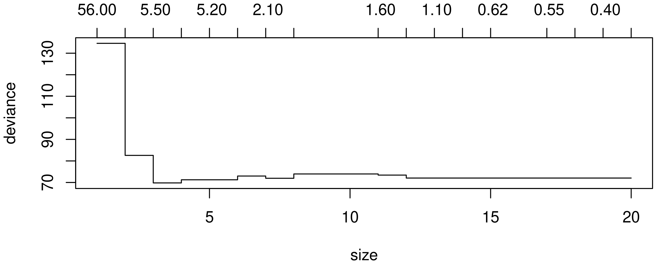
cv.tree() implements the cross-validation of the previous slide and plot() draws the summed out-of-fold deviance against size (bottom axis) and k (top axis).
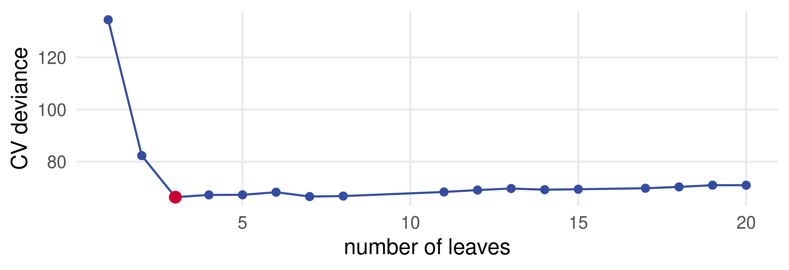
The deviance drops sharply up to three leaves and barely moves after that. The minimum is at three.
The curve is exactly flat from 12 leaves up. That is not evidence that big trees do equally well, as the next slide explains.
A caveat about cv.tree()
cv.tree() grows each fold’s tree with the default stopping rules, whatever options built the tree you pass it. On the prostate data a default tree has about nine leaves, so a fold tree “pruned” at a small k is just the whole fold tree, evaluated again and again: that is the flat segment.
Warning
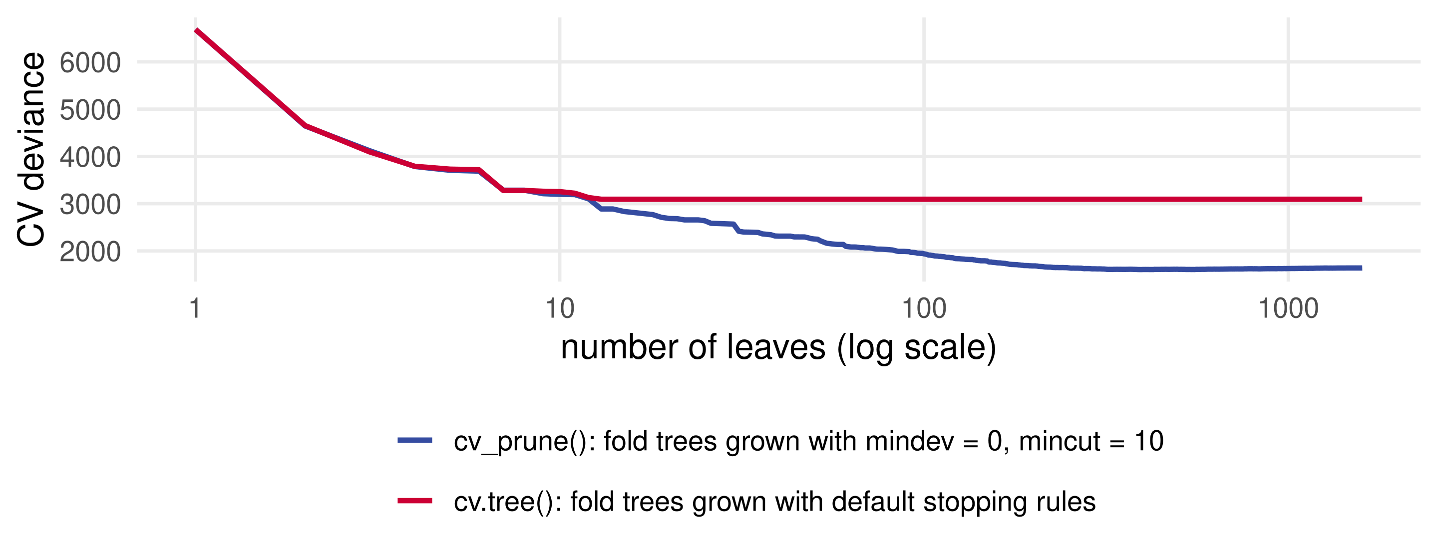
cv.tree() never evaluates subtrees larger than a default-grown tree. With mindev = 0 trees of hundreds of leaves, its curve goes flat at a few dozen leaves and the “best” size it reports is wrong.
The fix is to write the cross-validation loop ourselves, growing every fold’s tree with the same options as the full tree.
The algorithm, written out
Ten lines reproduce Algorithm 8.1 and pass the growing options to every fold through ...:
cv_prune <-function(formula, data, K =10, ...) { full <-tree(formula, data = data, ...) path <-prune.tree(full) # sizes and k of the full tree fold <-sample(rep(1:K, length.out =nrow(data))) dev <-0for (i in1:K) { t_i <-tree(formula, data = data[fold != i, ], ...) # same stopping rules as the full tree dev <- dev +prune.tree(t_i, newdata = data[fold == i, ], k = path$k)$dev }data.frame(size = path$size, k = path$k, dev = dev)}
prune.tree(t_i, newdata = ..., k = path$k) prunes the fold tree at every k of the full tree’s path and evaluates each subtree on the held-out fold.
Now the curve varies all the way up, and the minimum is still at three leaves. Here the two procedures agree; on the California tree they will not.
The pruned tree
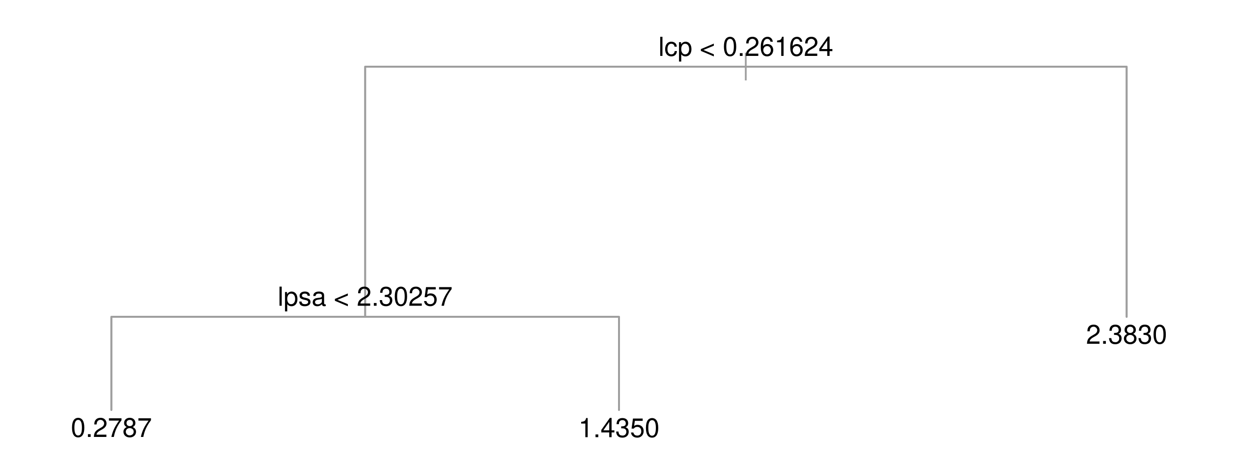
pstcut <-prune.tree(pstree, best = cvp$size[which.min(cvp$dev)])par(mar =c(1, 2, 1.5, 2), xpd =NA); plot(pstcut, col =8); text(pstcut, cex =0.9)
Three leaves summarize 97 patients: capsular penetration first, then PSA among the low-penetration patients. Age, hyperplasia and the Gleason score never enter the pruned tree, though all but the Gleason score appeared in the overgrown one.
Checkpoint: pruning
Why can a stopping rule based on the improvement from the next split fail, when pruning cannot?
In the genre path, what does k = 19.08 for the two-leaf subtree mean?
You pass a 1,500-leaf tree to cv.tree() and the curve is flat from 13 leaves up. What happened?
Random forests
Average many noisy trees instead of choosing one
Bagging: bootstrap aggregation
In lecture 10 the bootstrap measured sampling uncertainty:
for b = 1, \dots, B, resample n observations with replacement;
compute the estimator \hat\beta^*_b on each resample;
use the spread of \hat\beta^*_b across b for standard errors and confidence intervals.
Bagging (Breiman, 1996) uses the same resamples to build a new estimator, their average:
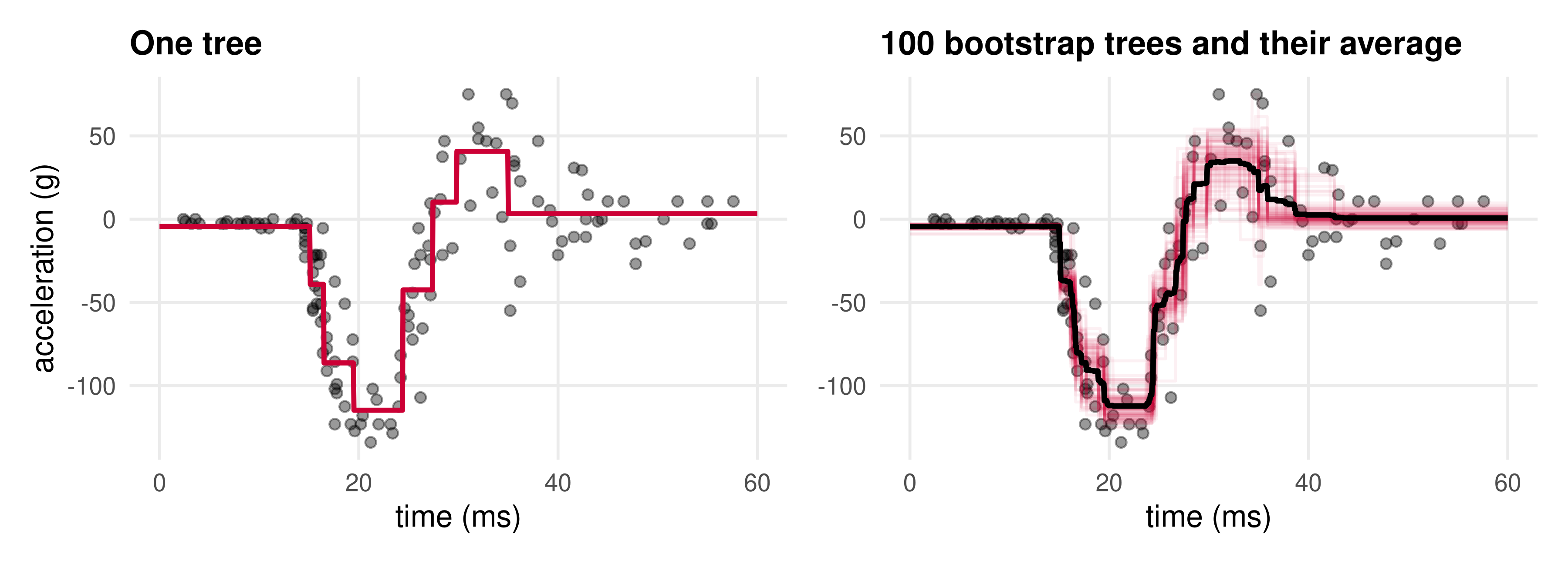
Each resample grows its own tree, with its own cutpoints. The bagged predictor averages the 100 step functions pointwise.
One tree against a hundred
Cutpoints jump around from resample to resample: trees have high variance. Averaging smooths the jumps away.
Bagging is model averaging. It lowers variance and leaves the bias of the individual trees roughly alone.
From bagging to random forests
A random forest (Breiman, 2001) is bagging applied to trees with one more source of randomness.
At every split of every bootstrap tree, choose the best split among a random subset of m of the d covariates rather than all d. With m = d the forest is plain bagging.
Why? If one covariate dominates, every bagged tree splits on it first and the trees are highly correlated, so averaging them removes little variance. Restricting the candidates decorrelates the trees. It also lets a tree take a split that is greedily suboptimal but pays off later, as in the checkerboard.
The cost is more randomness in each tree, which the average removes.
Forests do well without much tuning:
m is the main parameter; the default m = \lfloor\sqrt{d}\rfloor (regression software often uses d/3) usually works;
each tree is grown nearly to the bottom (ranger’s default minimum node size is 5 for regression, 1 for classification), because overfitting a single tree is harmless once it is averaged;
more trees never hurt; a few hundred is typical.
The random forest algorithm
Adapted from Hastie, Tibshirani and Friedman (2009), Algorithm 15.1.
For b = 1, \dots, B:
draw a bootstrap sample of size n from the data;
grow a tree T_b on it: at each node, pick m covariates at random, find the best split among them, and split; stop when a node reaches the minimum size.
Output the ensemble \{T_b\}_{b=1}^B.
Prediction at x:
regression: \hat f_{\text{RF}}(x) = \frac{1}{B}\sum_b T_b(x), the average of the tree predictions;
classification: the majority vote of the B trees, or the average of their class shares.
What a forest gives up, and what it gives back
No tree to draw. The forest is an average of hundreds of trees, so the dendrogram is gone and the recursive-partition picture with it.
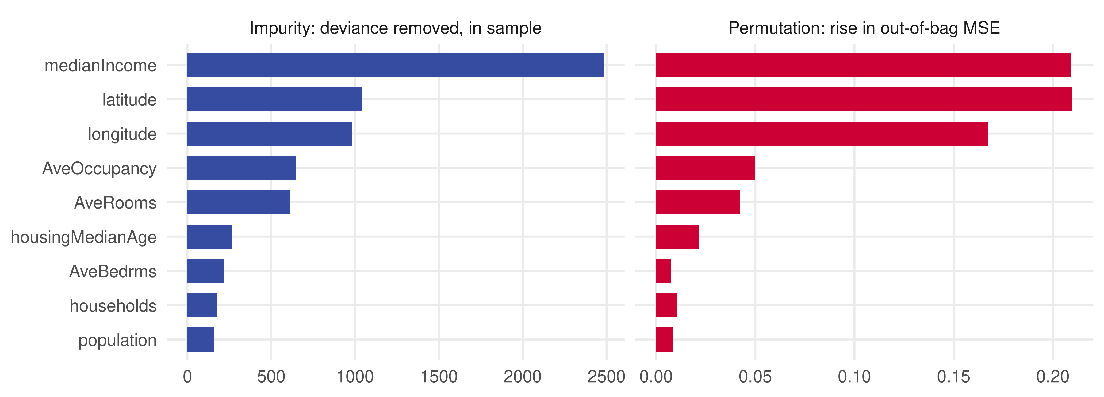
Variable importance partly replaces it: for each covariate, add up the deviance removed by every split on that covariate, over all trees. A second measure, permutation importance, shuffles one covariate in the data not used by each tree and records how much the prediction error rises.
Out-of-bag error for free. Each bootstrap sample leaves out about 37 percent of the observations (“out of bag”). Predicting each observation from the trees that did not see it gives an honest error estimate with no extra fitting, a built-in cross-validation.
California housing
Median house value for 20,640 census block groups (the book says tracts; the count says block groups), with location, income, age and household composition. We make per-household variables and take logs.
CAhousing <-read.csv("data/CAhousing.csv")CAhousing$AveBedrms <- CAhousing$totalBedrooms / CAhousing$householdsCAhousing$AveRooms <- CAhousing$totalRooms / CAhousing$householdsCAhousing$AveOccupancy <- CAhousing$population / CAhousing$householdslogMedVal <-log(CAhousing$medianHouseValue)CAhousing <- CAhousing[, -c(4, 5, 9)] # drop the room totals and the value in levelsCAhousing$logMedVal <- logMedValnames(CAhousing)
Nine covariates, so a forest’s default is m = \lfloor\sqrt{9}\rfloor = 3 candidates per split.
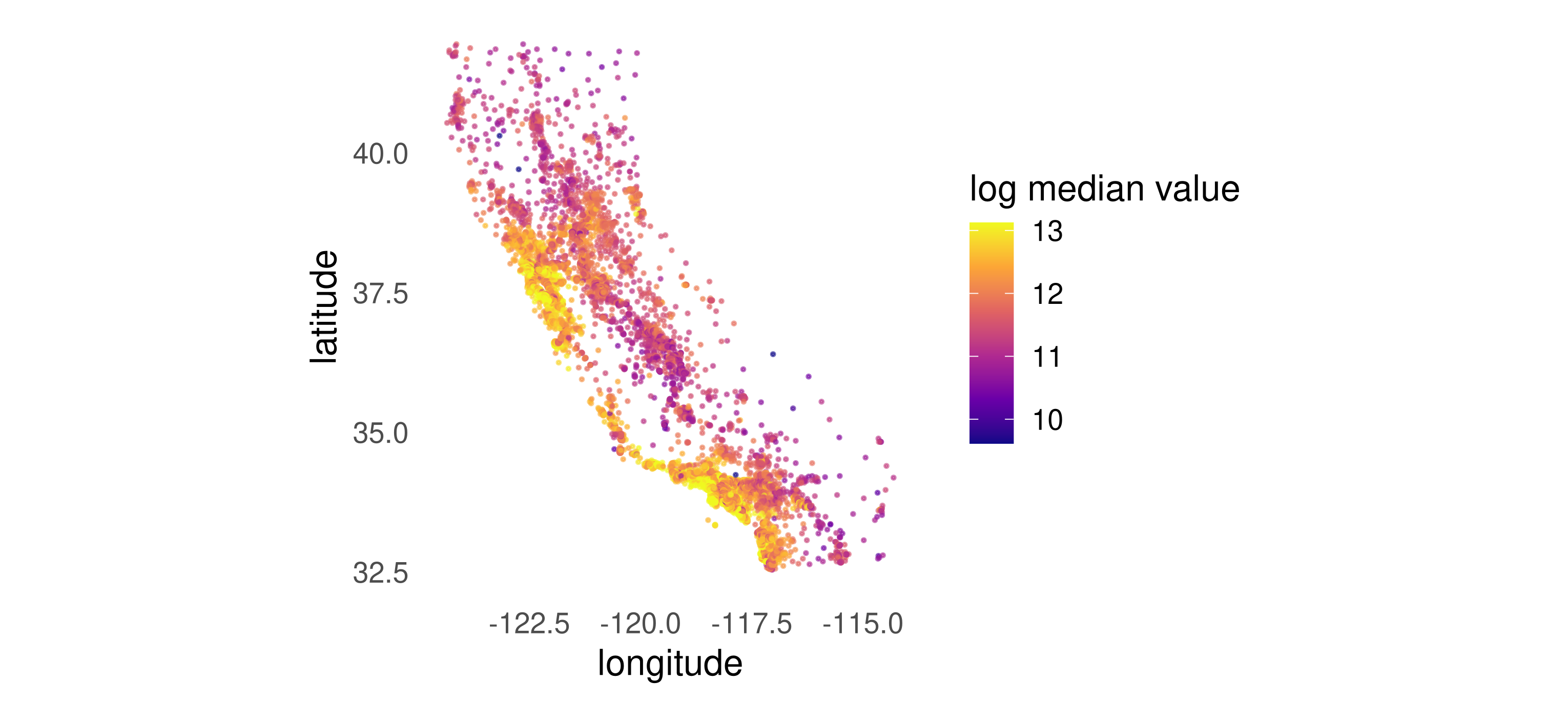
Where the expensive housing is
Value is a function of where you are: the Bay Area and the coast from Santa Barbara to San Diego are expensive, the Central Valley is not. A tree finds such pockets with a few splits on longitude and latitude; a linear model in longitude and latitude cannot.
## Ranger result
##
## Call:
##  ranger(logMedVal ~ ., data = CAhousing, num.trees = 200, min.node.size = 5,      importance = "impurity")
##
## Type:                             Regression
## Number of trees:                  200
## Sample size:                      20640
## Number of independent variables:  9
## Mtry:                             3
## Target node size:                 5
## Variable importance mode:         impurity
## Splitrule:                        variance
## OOB prediction error (MSE):       0.05255512
## R squared (OOB):                  0.8377498
Variable importance
Income and location dominate on both measures; the permutation measure, computed out of bag, puts latitude level with income. Household counts matter little once the per-household ratios are in.
Two rivals: a lasso and a pruned tree
Lasso. Standardize, interact everything with longitude and latitude (31 columns), and cross-validate.
set.seed(0)XXca <-model.matrix(logMedVal ~ . * longitude * latitude, data =data.frame(scale(CAhousing)))[, -1]capen <-cv.glmnet(x = XXca, y = logMedVal, alpha =1, lambda.min.ratio =1e-4)sum(coef(capen, s ="lambda.min")[-1] !=0) # nonzero coefficients at lambda.min
## [1] 21
Pruned tree. Overgrow with leaves of at least ten block groups, then cross-validate the pruning path.
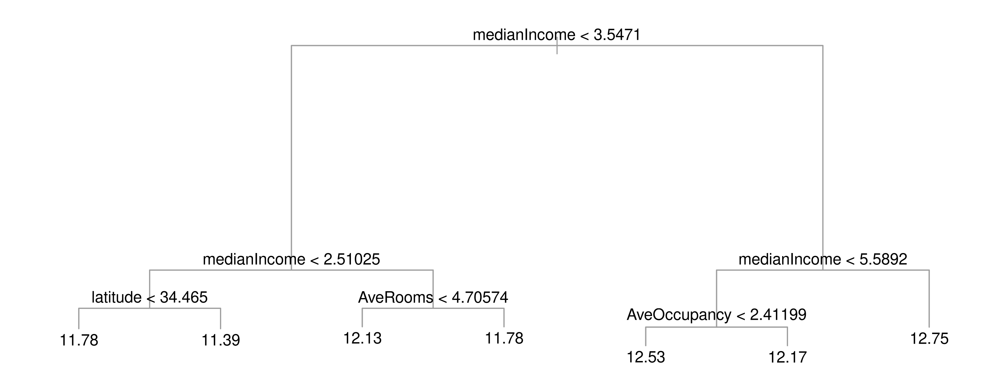
catop <-prune.tree(catree, best =7)par(mar =c(1, 2, 1.5, 2), xpd =NA); plot(catop, col =8); text(catop, cex =0.85)
Income first and income again at both ends; latitude for the poorest block groups and the per-household ratios in the middle. The chosen tree continues for another 390 leaves, most of them splits on longitude and latitude.
Head to head, out of sample
Ten random splits: fit on 5,000 block groups, predict the other 15,640, compute the RMSE of log value. This is the code behind the opening figure.
One block group has an average occupancy of 1,243 persons per household (the next largest is 600). Standardized and interacted with longitude and latitude, it sits far outside the training range whenever it is in the test set, and the linear fit extrapolates to log-value errors of 50 to 170.
A tree only asks whether occupancy exceeds a threshold, so an extreme covariate value cannot produce an extreme prediction. Trees are invariant to monotone transformations of the covariates and immune to outliers in X; linear models are neither.
Even dropping the sixteen worst test errors, the lasso’s RMSE is about 0.33: no better than the pruned tree and well above the forest.
Where the forest’s gain comes from
Trees find pockets. A few splits on longitude and latitude isolate the Bay Area and coastal Los Angeles. The lasso, with location entered linearly and through interactions, has no way to carve out a rectangle.
Averaging removes the tree’s variance. The pruned tree’s cutpoints and leaf means jump from sample to sample; the forest averages 200 of them.
No tuning parameter was chosen. The pruned tree needed cross-validation to pick about 160 leaves on 5,000 observations; the forest used defaults.
Could the lasso find cutpoints? Yes, with cleverly defined indicator variables (Wang, Sharpnack, Smola and Tibshirani, 2016, do this for trend filtering), but trees do it automatically.
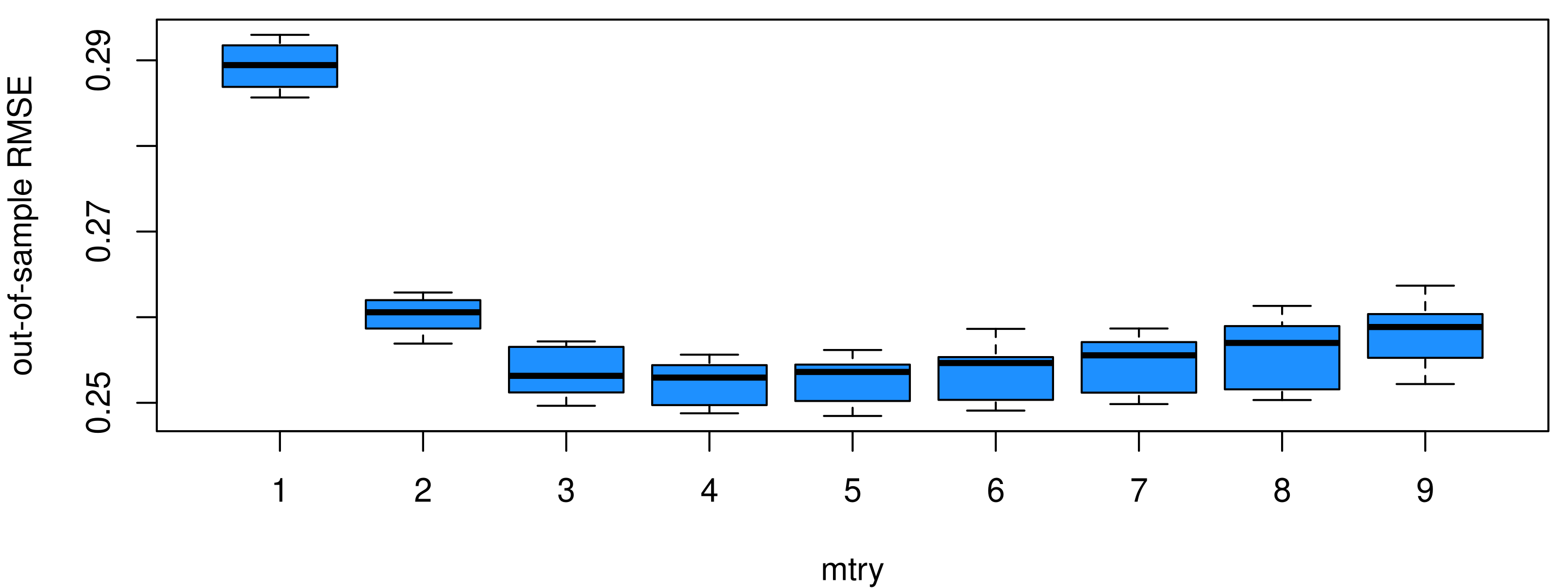
mtry = 1 (a random covariate at every split) is clearly worse and mtry = 2 slightly so. From 3 to 9 the curve is flat within the noise of the ten splits, with the minimum at 4.
The default \lfloor\sqrt{9}\rfloor = 3 is as good as anything, which is the folk wisdom: forests “typically work well” out of the box.
Every value of mtry, including plain bagging at mtry = 9, beats the pruned tree and the lasso.
Checkpoint: random forests
Bagging averages B trees. Why does it reduce variance and not bias?
What does mtry change, and why can a smaller mtry lower the error of the average even though it raises the error of each tree?
What is the out-of-bag error, and why is it an honest estimate?
Trees and forests in one page
A tree is an adaptive binned sample mean. Recursive binary splits choose which covariate to cut, where, and how finely; the leaves are the bins and the fit is a step function.
Growing is greedy, so do not stop early. Each split minimizes the deviance one step ahead. A near-useless split can precede a decisive one, so overgrow the tree and prune it back.
Prune by weakest link, choose by cross-validation. Cost-complexity pruning yields a nested path indexed by the number of leaves; cv.tree() evaluates it, but only up to the size of a default tree, so write the loop yourself for big trees.
Forests average many overgrown trees. Bagging removes the tree’s variance; random covariate subsets decorrelate the trees; the out-of-bag error comes free. The defaults usually work, and on the California data the forest beat both the pruned tree and the lasso in every split.
Trees are robust to the scale of X, linear models are not. A single extreme covariate value sank the lasso and left the trees untouched.
Taddy, Business Data Science (2019), chapter 9: the TV, prostate and California data.
Athey and Imbens (2019) survey machine learning methods for economists, and Wager and Athey (2018) turn forests into estimators of heterogeneous treatment effects, the topic of a later lecture.
Additional derivations and code
Optional material for reference and practice
Why averaging correlated trees helps
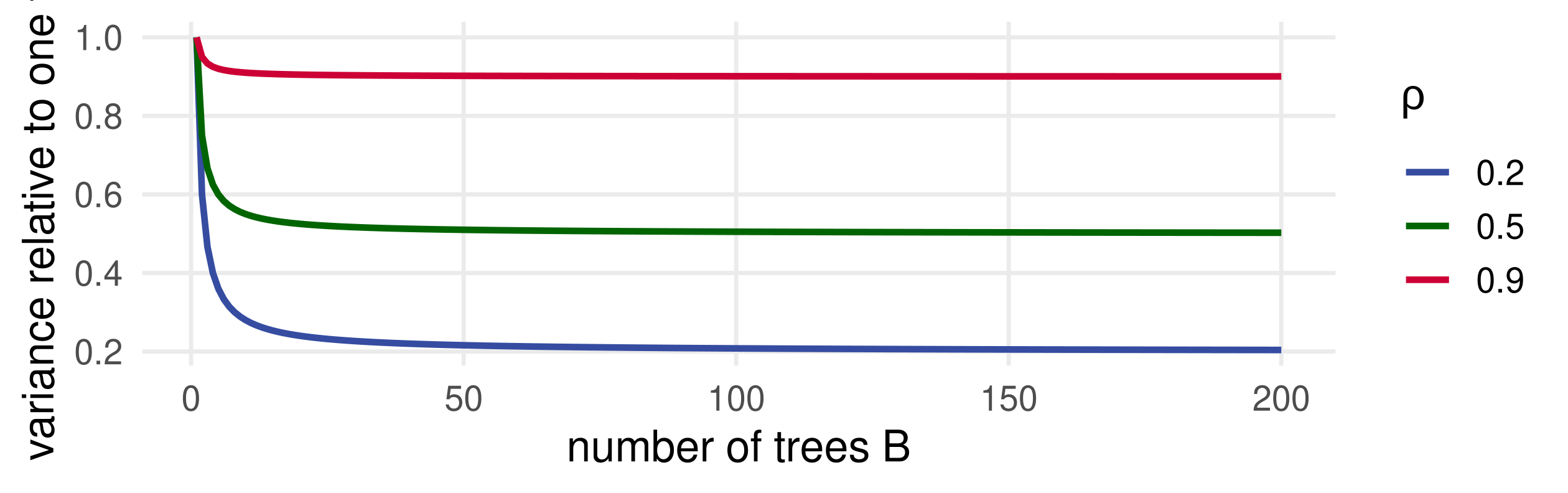
Let B tree predictions at a point be identically distributed with variance \sigma^2 and pairwise correlation \rho. The variance of their average is
The second term vanishes as B grows; the first, \rho\sigma^2, is a floor that more trees cannot breach. The random covariate subset lowers \rho and so lowers the floor: that is the whole point of mtry (Hastie, Tibshirani and Friedman, section 15.2).
Out of bag
A bootstrap sample draws n times with replacement. The chance that a given observation is never drawn is
n <-nrow(CAhousing)c(exact = (1-1/ n)^n, limit =exp(-1))
##     exact     limit
## 0.3678705 0.3678794
set.seed(0)mean(!(1:n %in%sample.int(n, replace =TRUE))) # share out of bag in one resample
## [1] 0.3704942
Each tree sees about 63 percent of the observations and leaves 37 percent out, so with B = 200 every observation is out of bag for about 74 trees. The out-of-bag prediction for observation i averages those trees, and the resulting error is the OOB prediction error that ranger() printed (MSE 0.0526, R^2 0.838).
Weakest-link pruning in formulas
For a subtree T of the big tree T_0 with leaves m = 1, \dots, |T|, write the deviance R(T) = \sum_m \sum_{i \in R_m} (Y_i - \bar Y_m)^2 and the cost-complexity criterion R_\alpha(T) = R(T) + \alpha |T|.
For an internal node t, let T_t be the branch below it. Collapsing T_t into the single leaf t raises the deviance by R(t) - R(T_t) and removes |T_t| - 1 leaves. The link strength is g(t) = \frac{R(t) - R(T_t)}{|T_t| - 1}.
Collapse the node with the smallest g(t), recompute, repeat. The values of g at each collapse are increasing: \alpha_1 < \alpha_2 < \cdots, and the subtree obtained at step k minimizes R_\alpha(T) for every \alpha \in [\alpha_k, \alpha_{k+1}).
Breiman et al. (1984) prove the sequence is nested and that each member has the smallest R(T) among subtrees of T_0 with its number of leaves.
The k column of prune.tree() is (\alpha_1, \alpha_2, \dots): in the genre path, g = 7.606 for node 5 (deviance 7.606, two pure children, one leaf removed), then 16.22 for node 3, then (33.42 - 14.34)/1 = 19.08 for node 2, then (75.80 - 49.64)/1 = 26.16 for the root.
Node impurity for classification
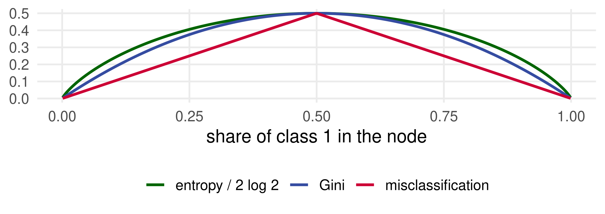
For a node with class shares p_1, \dots, p_K, three measures of how mixed it is:
Measure
Formula
In tree()
Misclassification error
1 - \max_k p_k
not used for splitting
Gini impurity
\sum_k p_k(1 - p_k)
split = "gini"
Entropy (the deviance is 2n \times entropy)
-\sum_k p_k \log p_k
default
Gini and entropy are strictly concave, so they reward a split that purifies the children even when the majority class does not change; misclassification error does not, which is why trees are not grown with it.
Trees as adaptive basis functions
A tree with leaves R_1, \dots, R_M is the regression
a linear model in M indicator variables whose definition is chosen by the data. Two consequences:
Invariance. Only the ordering of each covariate matters, so replacing X_j by any increasing transformation, \log X_j or its rank, leaves the tree unchanged. The lasso in section 4 was wrecked by a covariate value of 1,243; the tree did not notice.
Roughness. The fit is piecewise constant and jumps at the thresholds, so it is poor at smooth relationships; bagging and forests smooth the jumps (the motorcycle picture), and boosting, not covered today, adds trees sequentially to fix the residuals.
The lasso can mimic a tree if the analyst supplies the indicators: Wang et al. (2016) penalize differences of neighbouring fitted values on a grid, which selects cutpoints. Trees find the cutpoints themselves.
cv.tree() against the written-out loop on the California tree
nbc_showdetails.csv and nbc_demographics.csv, the 40 TV shows and their audience shares;
prostate.csv, the 97 prostate cancer patients;
CAhousing.csv, the 20,640 California block groups.
MASS::mcycle ships with R. The notes use the same packages; randomForest is the older alternative to ranger.
Return to the question
Three predictors of California house prices: the lasso extrapolated off a single block group, the pruned tree needed cross-validation to find its 160 leaves, and the random forest, two hundred overgrown trees averaged, won every split with the defaults. Trees pick the bins; forests average the trees.