ECON 4370 / 6370 Computing for Economics

Lecture 12: Regularized Regression

Zhan Gao

08 October 2026

A thousand regressors, ten thousand households

Predict a household’s online spending from the share of its browsing time at each of 1,000 websites. Fit on 8,000 households, test on 2,000 others.

model	sites_used	in_sample_r2	out_of_sample_r2
OLS, all 1,000 sites	999	0.282	-0.097
Lasso, lambda.min	228	0.177	0.107
Lasso, lambda.1se	86	0.125	0.100

• OLS uses every site and fits the training sample best, yet it predicts new households worse than their average: its out-of-sample R^2 is negative.
• The lasso keeps a few hundred sites, or under a hundred, and predicts better.

Last lecture’s lesson was that complexity must be chosen out of sample. Today’s tool, regularization, generates the candidates to choose from and makes 1,000 regressors manageable.

Same split as the “Does it beat OLS” slide in section 3, where the code is shown. OLS has one NA coefficient (a site with no visits in the training households), set to zero for prediction. The in-sample R-squared of OLS is 0.28 against 0.13 for the lasso; the gap is overfitting.

Today’s route

1. Why regularize: too many candidate models, and a penalty that tames them.
2. Lasso and ridge: two cost functions, why one of them selects variables, and the regularization path.
3. Online spending with glmnet: a sparse design matrix, the path, cross-validation and prediction.
4. Practical details: folds, the one-standard-error rule, factors and standardization.
5. Beyond the lasso: the elastic net and the group lasso.

Additional derivations and code follow the main lesson.

Lecture 11 built the recipe: candidates indexed by a tuning parameter, CV error for each, pick the minimum or the one-SE choice. Today the tuning parameter is the penalty lambda. The next lecture (trees) uses the same recipe with tree depth.

Packages and data

Run the examples from the lectures/ directory.

library(tidyverse)
library(Matrix)   # sparse matrices
library(glmnet)   # lasso, ridge and elastic net paths, with cross-validation

File	Role
data/browser-totalspend.csv	Online spending of 10,000 households
data/browser-domains.csv	Visits by household and website, 2.3 million rows
data/browser-sites.txt	The names of the 1,000 websites
data/oj.csv	Orange juice sales, for the factor-coding example

[Sources] - The browser data are the comScore household browsing panel as distributed with Taddy, Business Data Science (2019); the notes follow that treatment. glmnet also fits logistic, Poisson and Cox models with the same penalties through the family argument.

Why regularize

---

Cross-validation needs candidates, and with many regressors there are too many

Cross-validation needs a set of candidates

• Last lecture: given candidate models, K-fold CV picks the one with the best estimated out-of-sample performance.
• For the binned sample mean the candidates were manageable: one per number of bins, a few thousand at most.
• Even with a single regressor there are many other candidate families: bins cut in other ways (regression trees, next lecture), polynomials, Fourier series, wavelets.
• With d regressors the natural candidate set is every subset of them, and that set explodes.

Subsets explode

Regressors d	Subsets 2^d
10	1,024
20	1,048,576
50	about 10^{15}
100	about 10^{30}

• For d = 100 there are more candidate models than 16-digit passwords, so checking them all takes longer than a brute-force password attack.
• Typical high-dimensional data have d in the thousands. The browsing data have 1,000 sites, and interactions would multiply that.
• We need a structured family of candidates that is cheap to generate and indexed by a single tuning parameter.

High-dimensional problems

When the number of parameters p is large relative to the sample size n:

• If p \ge n, the design matrix X has a nonzero null space, so the least squares solution is not unique: if \hat\beta minimizes \lVert y - X\beta \rVert^2, so does \hat\beta + v for every v with Xv = 0.
• Even with p < n, OLS with many regressors has high variance and overfits, which is the pattern on the opening slide.
• For logistic regression the MLE may not exist at all: with enough regressors the classes can be separated perfectly.
• A thousand coefficients are hard to interpret. Simpler, structured solutions are easier to read.

Add a penalty to the deviance

Regression models are estimated by minimizing an in-sample deviance: the sum of squared errors for OLS, -2 \log \text{likelihood} for maximum likelihood.

Regularization adds a penalty for model complexity:

\text{dev}_{IS}(\beta) + \underbrace{\lambda \sum_{j=1}^d c(\beta_j)}_{\text{penalty}},

• c(\beta_j) \ge 0 is a cost attached to the size of \beta_j, and \lambda \ge 0 is the penalty parameter that says how much complexity costs.
• We choose c(\cdot) and \lambda, then minimize the regularized objective instead of the deviance alone. The minimizer is a new, regularized estimator, one for every value of \lambda.

\lambda is a complexity dial

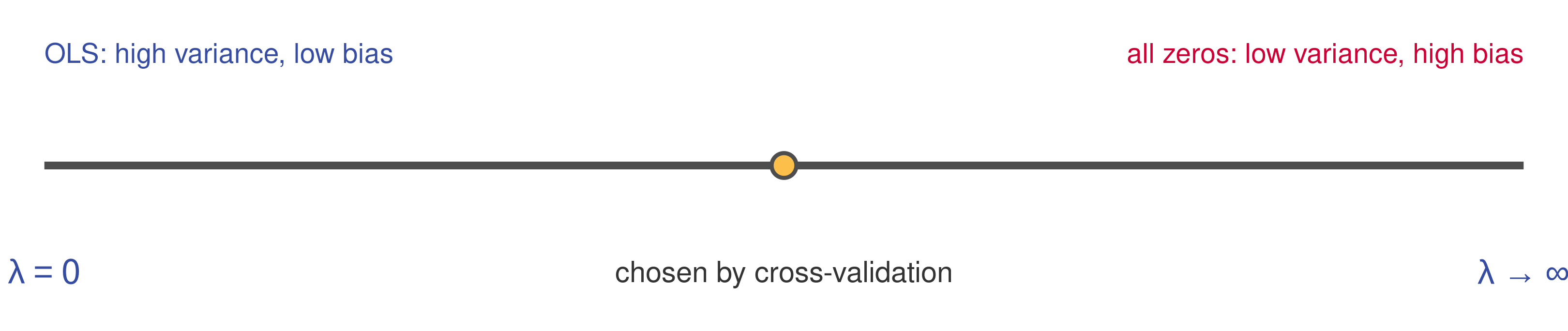
• \lambda = 0 gives the original estimator. As \lambda \to \infty only the penalty matters, and with c increasing in |\beta_j| the minimizer is \hat\beta = 0.
• A \hat\beta closer to zero is a less complex model: the prediction \hat{\mathbf{E}}[Y \mid X] = G(X'\hat\beta) varies less across values of X.
• The penalty asks the computer to fit the data but to prefer the simpler model when two fit about equally well. This is the parsimony principle, and \lambda sets the exchange rate.

The constrained view

Minimizing the penalized objective is equivalent to a constrained problem:

\min_\beta\ \text{dev}_{IS}(\beta) \quad \text{subject to} \quad \sum_{j=1}^d c(\beta_j) \le s.

• Minimize the deviance, but do not let the total cost exceed the budget s.
• s plays the opposite role of \lambda: a large s makes the constraint irrelevant (OLS), while s = 0 forces the least complex model.
• Every \lambda > 0 corresponds to some budget s, and this view is what makes the geometry on the next slides possible.

Checkpoint: regularization

1. With 30 candidate regressors, how many subset models are there? Could you cross-validate them all?
2. Why does a large \lambda reduce variance, and what does it cost?
3. If c(\beta_j) = \beta_j^2 and you double \lambda, does the penalized estimator become more or less complex?

Answers: 2^30, about one billion, so no; the estimator moves less across samples because it is pulled toward a fixed point, zero, but it is pulled away from the truth, which is bias; less complex, since the cost of any nonzero coefficient doubles.

Lasso and ridge

---

Two cost functions, and why one of them selects variables

Two cost functions

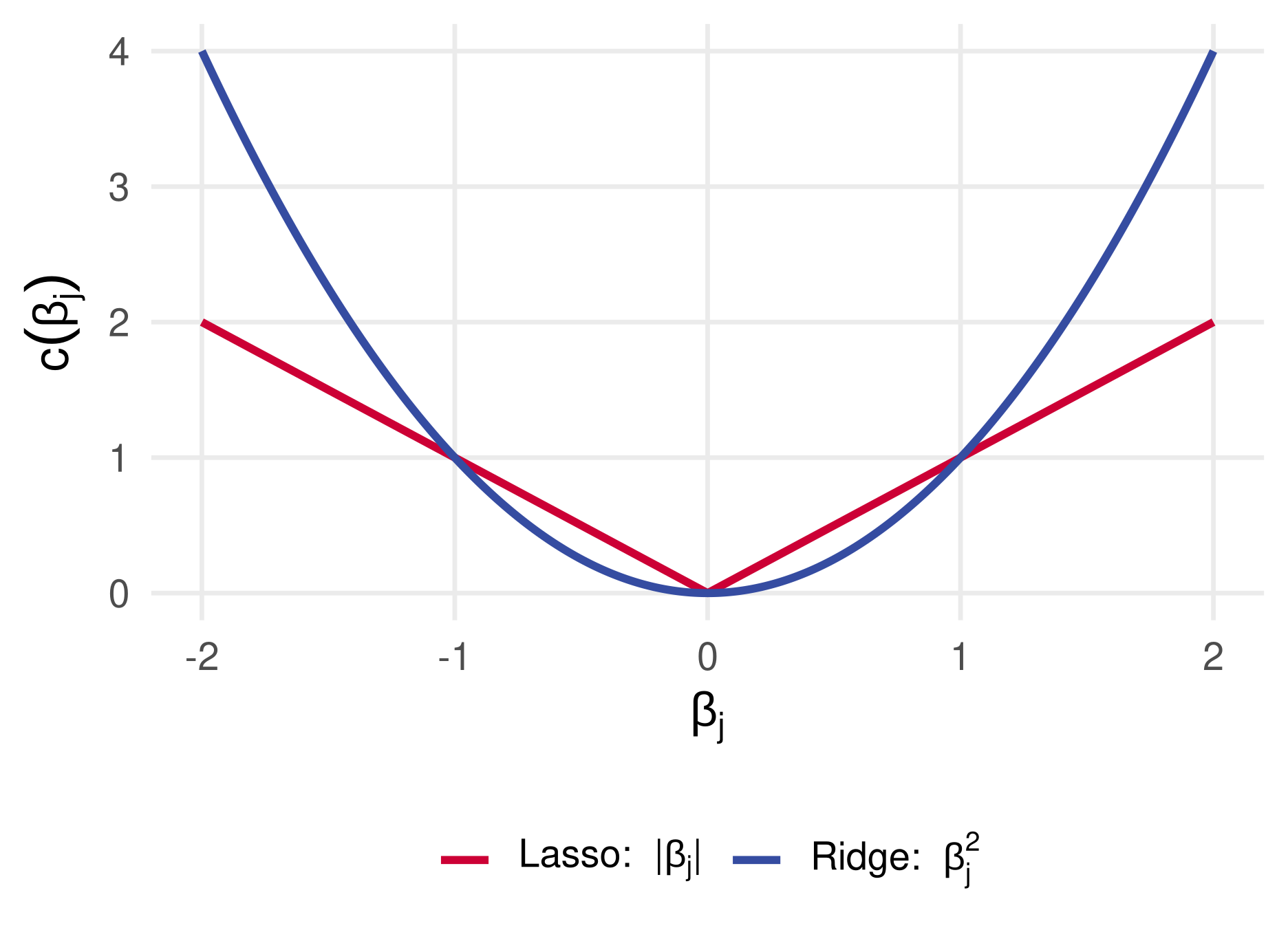
Both costs are zero at zero and increase in |\beta_j|, so the cheapest model is the least complex one.

• Lasso: c(\beta_j) = |\beta_j|. Moving \beta_j by x units costs x, near zero or far from it.
• Ridge: c(\beta_j) = \beta_j^2. The cost grows faster the larger \beta_j is, and is nearly flat near zero.
• The lasso penalty is the \ell_1 norm \sum_j |\beta_j| (the “Manhattan” norm). Ridge uses the squared \ell_2 or Euclidean norm \sum_j \beta_j^2.
• Many other costs are possible. These two dominate because they have useful theory and are easy to compute for the workhorse deviances.

[Sources] - Tibshirani (1996), Regression shrinkage and selection via the lasso, JRSS-B 58, 267-288. - Hoerl and Kennard (1970) introduced ridge regression.

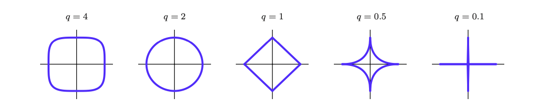
Contours of |\beta_1|^q + |\beta_2|^q

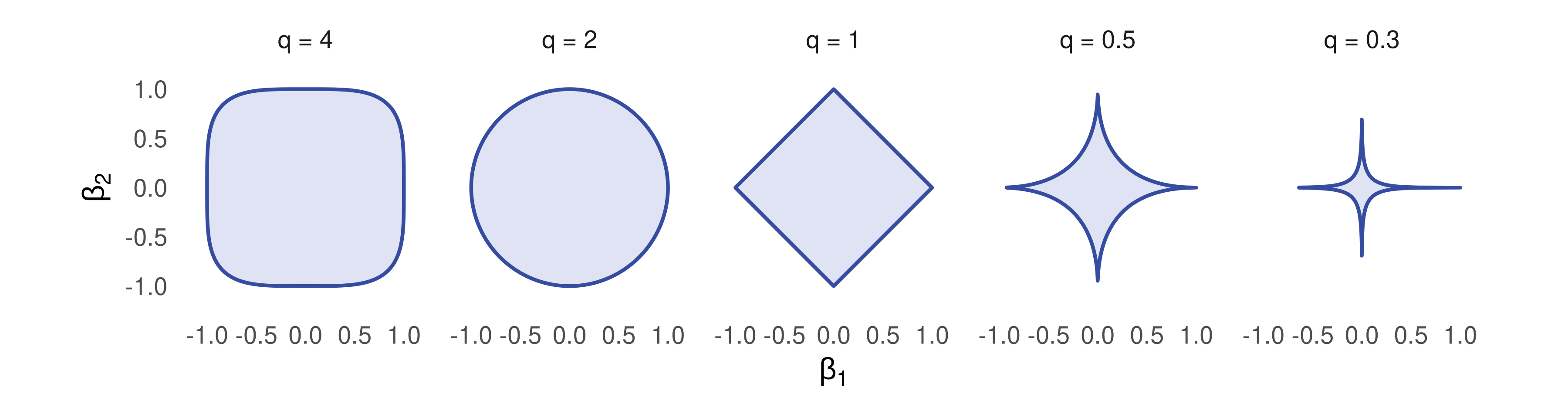
• q = 2 is ridge, q = 1 the lasso. The set \{\beta: |\beta_1|^q + |\beta_2|^q \le s\} is the constraint region of the previous slide.
• The lasso region has corners on the axes, where one coefficient is exactly zero. The ridge disc has none.
• q < 1 is even spikier but not convex, which makes the optimization hard (see computation below).

[Sources] - Hastie, Tibshirani and Friedman (2009), The Elements of Statistical Learning, figure 3.12, which the notes reproduce as images/lq_balls_hastie_et_al_2009.png.

Why the lasso sets coefficients exactly to zero

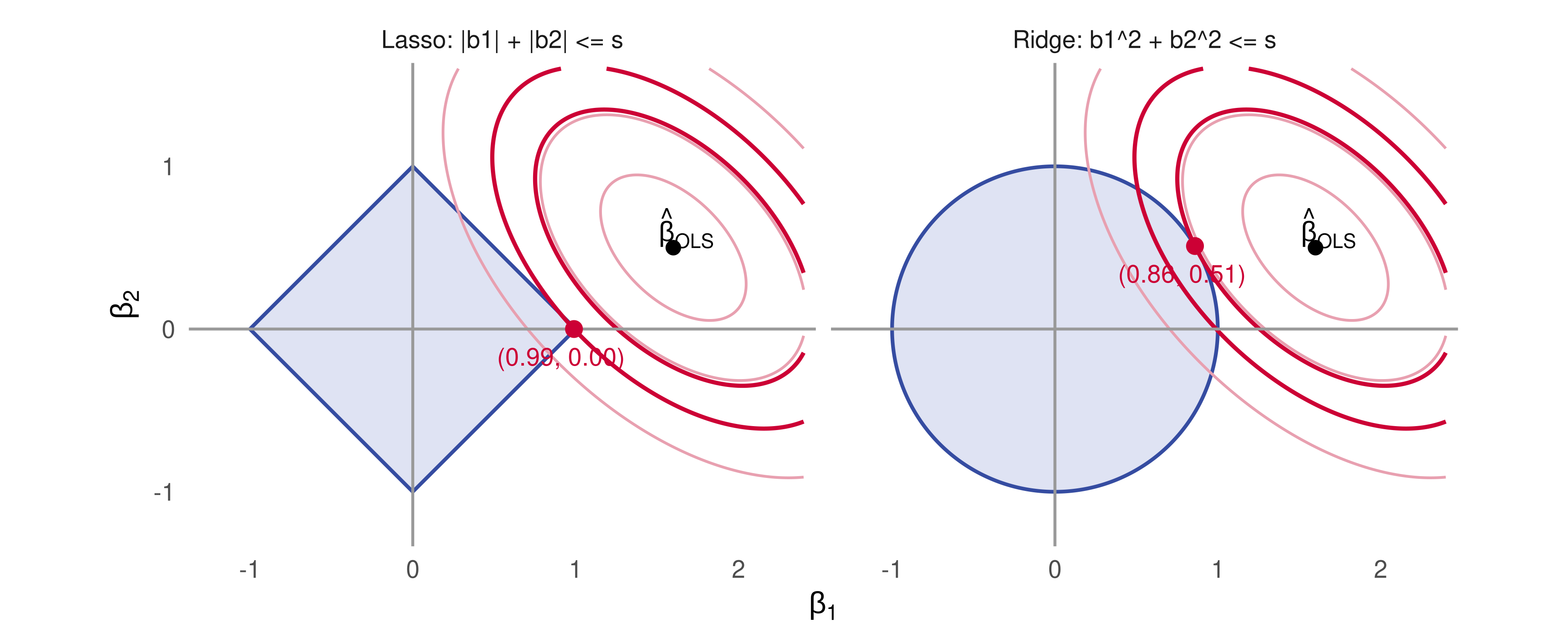
Both constrained solutions sit where the smallest reachable deviance contour touches the constraint region. The lasso’s touches at a corner.

Reading the picture

• Blue areas are the constraint regions, the \beta’s with c(\beta_1) + c(\beta_2) \le s.
• Red ellipses are contours of the deviance: pairs (\beta_1, \beta_2) with the same sum of squared errors. Their center is the unconstrained OLS estimate, and ellipses further out have higher deviance.
• The constrained solution is the point of the region on the lowest contour it can reach. It has higher deviance than OLS, but it satisfies the budget.
• With a spiky region the lowest contour usually lands on a corner, where one coefficient is exactly zero: the lasso selects a smaller model. The ridge disc has no corners, so ridge coefficients are shrunk but almost never exactly zero.
• Relative to OLS both solutions are closer to the origin: both penalties shrink.

[Sources] - James, Witten, Hastie and Tibshirani, An Introduction to Statistical Learning, figure 6.7, which the notes reproduce as images/penalties2.png. Here the deviance is the quadratic (b - b_ols)’ A (b - b_ols) with A = [1, 0.5; 0.5, 1] and b_ols = (1.6, 0.5), and the solutions are found by grid search within each region.

Shrinkage versus selection, in formulas

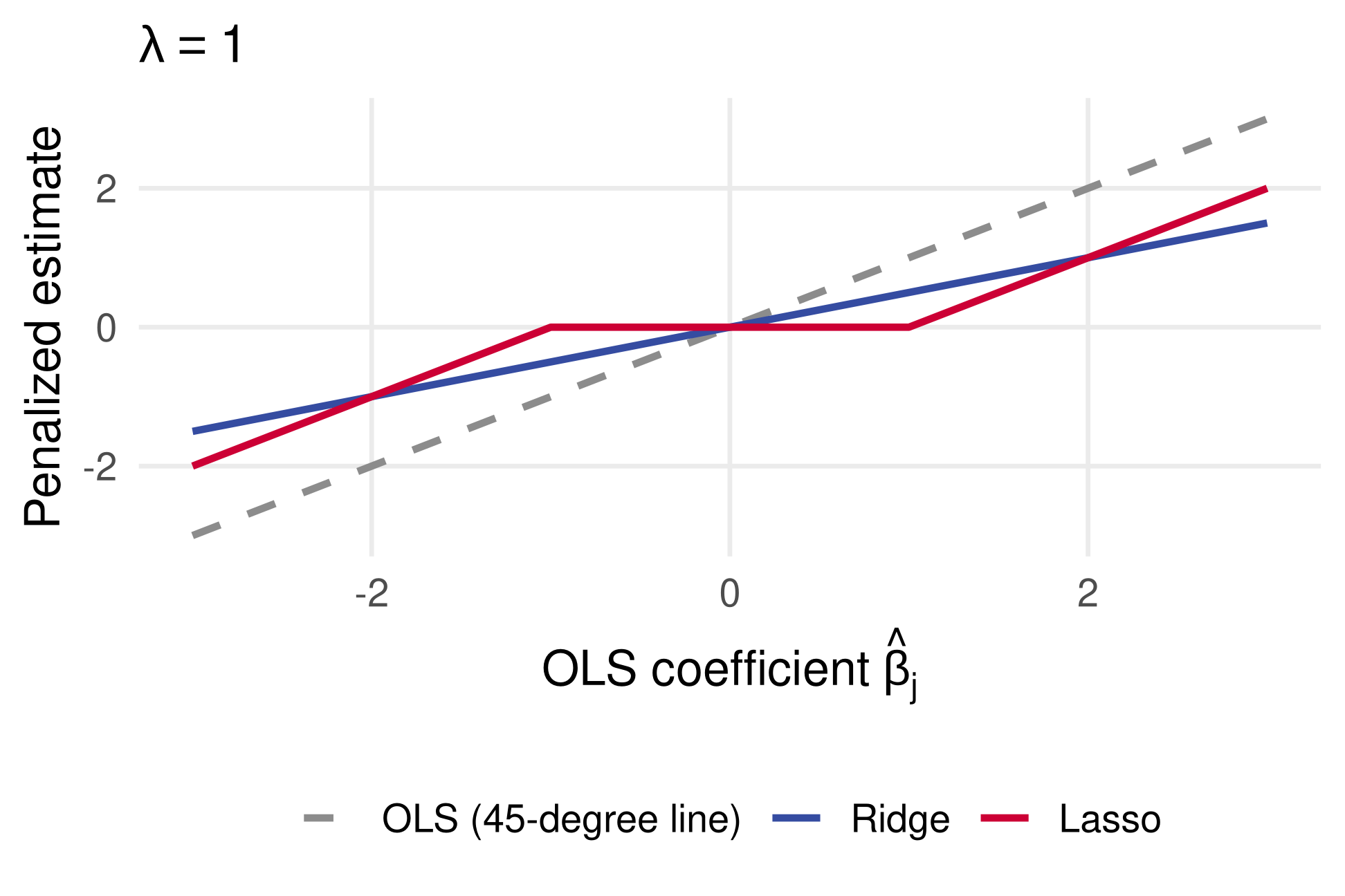
When the columns of X are orthonormal (X'X = I, so the OLS coefficients are \hat\beta_j = X_j'y), the two estimators have closed forms, coefficient by coefficient:

\hat\beta_j^{\text{ridge}} = \frac{\hat\beta_j}{1 + \lambda}, \qquad \hat\beta_j^{\text{lasso}} = \text{sgn}(\hat\beta_j)\,\big(|\hat\beta_j| - \lambda\big)_+ .

• Ridge scales every coefficient by the same factor below one. Nothing is zero.
• The lasso subtracts \lambda from every |\hat\beta_j| and sets to zero whatever falls below \lambda: soft-thresholding.
• The derivation is a one-line calculus exercise for each j (appendix).

[Sources] - Hastie, Tibshirani and Friedman (2009), The Elements of Statistical Learning, table 3.4 and section 3.4.3. With glmnet’s scaling of the objective, (1/2n) RSS + lambda times the penalty, the lasso formula holds exactly when the columns have mean zero and sum of squares n; the appendix verifies it numerically.

Sparsity

• A coefficient vector \hat\beta = (\hat\beta_1, \dots, \hat\beta_d)' with mostly zeros is sparse.
• The lasso’s corners make its solutions sparse: it does variable selection and estimation in one step, and the resulting model is simpler and easier to interpret. That accounts for much of its popularity over ridge.
• A large body of theory (not covered here) shows that the lasso predicts well when the true coefficient vector is sparse: a few regressors matter, and the rest are noise.
• Ridge shrinks toward zero without selecting. It is the better choice when many regressors each contribute a little, which the elastic net section revisits.

Both penalties shrink. Only the lasso selects.

Computation

• The lasso and ridge penalties are convex, and convexity is what makes these problems easy: there is one minimum and fast algorithms find it. glmnet and gamlr have built-in solvers, so no optimization details are needed for this class.
• We could impose sparsity directly with the cost c(\beta_j) = \mathbf{1}\{\beta_j \ne 0\}, the \ell_0 penalty. But that is not convex, and solving it means checking the 2^d subsets again.
• Not every ML estimator is computationally nice. Deep neural networks (later in the course) are non-convex and in principle impossible to solve exactly, yet they work well with ad hoc optimizers thanks to massive parallelization and empirical evidence that the global minimum is not needed.

[Sources] - Boyd and Vandenberghe, Convex Optimization, free at https://web.stanford.edu/~boyd/cvxbook/; the R package CVXR gives a general modelling interface. - Gao (2021), the notes’ Rmosek implementation reference, for a solver-based approach.

The regularization path

Each \lambda gives a different lasso estimator. Which one? Generate a sequence of candidates and let cross-validation choose.

1. Start at \lambda_1, the smallest penalty for which \hat\beta^1 = 0.
2. For t = 2, \dots, T, set \lambda_t = \delta\,\lambda_{t-1} for some \delta \in (0, 1) and compute \hat\beta^t under penalty \lambda_t.

The sequence \hat\beta^1, \dots, \hat\beta^T is the lasso regularization path: it starts at the least complex model and adds complexity in small steps.

• glmnet() does this automatically, with T = 100 values by default, spaced so that \lambda_T is a small fraction of \lambda_1.
• Starting from the top is also computationally smart: each solution is a warm start for the next, slightly smaller \lambda.

Checkpoint: lasso and ridge

1. Two regressors are both useful and the OLS estimate is (2, 1.5). With a tight budget s, which estimator is more likely to drop one of them, lasso or ridge?
2. In the orthonormal case with \lambda = 1, what are the lasso and ridge estimates of an OLS coefficient equal to 0.6? Of one equal to 3?
3. Why does the path start at the largest \lambda rather than at \lambda = 0?

Answers: the lasso, because its corners put zeros on the boundary; lasso 0 and 2, ridge 0.3 and 1.5; the first solution is free (all zeros), each later one is a warm start, and the largest lambda is known in closed form from the data.

Online spending with glmnet

---

A sparse design matrix, the path, cross-validation and prediction

Three files

browser_spend <- read.csv("data/browser-totalspend.csv")   # one row per household
yspend <- browser_spend$spend
web <- read.csv("data/browser-domains.csv")                 # one row per household-site pair
sitenames <- scan("data/browser-sites.txt", what = "character", quiet = TRUE)
c(households = length(yspend), rows_in_web = nrow(web), sites = length(sitenames))

##  households rows_in_web       sites 
##       10000     2271684        1000

head(web, 3)

##     id site visits
## 1  991  873      1
## 2 7940  873      2
## 3 2453  873     12

• web records how many times each household (machine id) visited each site, with the sites numbered 1 to 1,000. Pairs with no visits are simply absent.
• 2,271,684 rows out of 1{,}000 \times 10{,}000 = 10{,}000{,}000 possible pairs: 77% of the entries are zero.

Turn the codes into factors

web$site <- factor(web$site, levels = 1:length(sitenames), labels = sitenames)  # site names
web$id <- factor(web$id, levels = 1:length(unique(web$id)))                     # household ids
head(web, 3)

##     id       site visits
## 1  991 032439.com      1
## 2 7940 032439.com      2
## 3 2453 032439.com     12

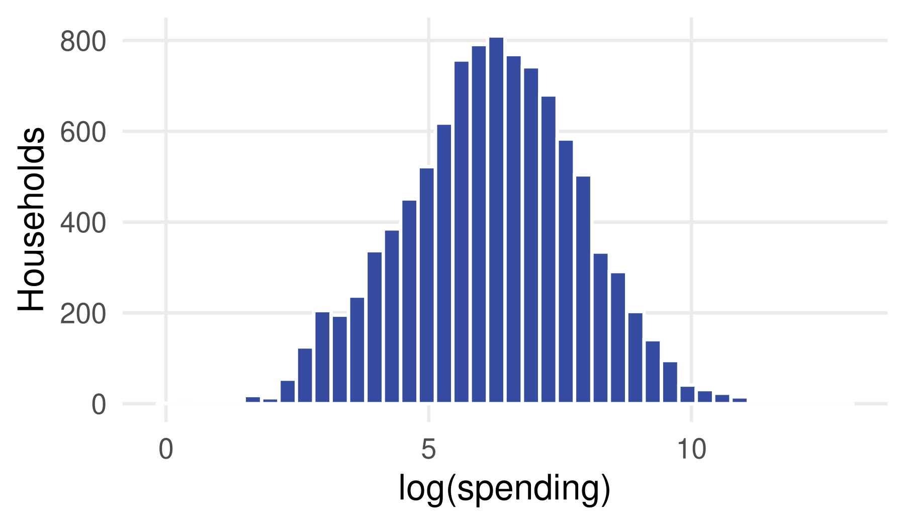
• Spending is heavily skewed: median 510, mean 1,946, maximum above 400,000. We model \log(\text{spend}).
• The outcome is a 10,000-vector and the regressors will be one column per site.

From visit counts to visit shares

We use the percentage of a household’s visits at each site rather than raw counts, so that heavy and light browsers are comparable.

machinetotals <- as.vector(tapply(web$visits, web$id, sum))   # total visits per household
visitpercent <- 100 * web$visits / machinetotals[web$id]      # share of that household's visits
head(visitpercent)

## [1] 0.02963841 0.01789709 0.13089005 0.01553760 0.08866558 1.03558652

• tapply(a, b, f) applies f to a within every level of the factor b, so machinetotals has one entry per household.
• Indexing machinetotals[web$id] uses the factor’s integer codes to line each row up with its household’s total.

The task: predict spending from browsing history. For that, each row of the design matrix must describe one household across all 1,000 sites.

Sparse matrices

A matrix with mostly zeros is sparse. A data frame or an ordinary matrix stores every zero, which wastes memory. A sparse format stores only the nonzero entries as triplets:

\begin{pmatrix} 40 & 0 \\ 0 & 100 \\ 60 & 0 \end{pmatrix} \quad \text{is stored as} \quad \begin{pmatrix} i = 1, 2, 3 \\ j = 1, 2, 1 \\ x = 40, 100, 60 \end{pmatrix}.

• sparseMatrix(i, j, x) in the Matrix package builds the matrix from triplets, which is exactly the form of web.
• From a data frame of covariates, sparse.model.matrix(~ x2 + x3 + x4, data = mydata) does the same job as model.matrix() but returns a sparse result.
• glmnet() and gamlr() take a model matrix and an outcome vector rather than a formula and a data frame, and both accept sparse matrices directly.

Build the design matrix

xweb <- sparseMatrix(i = as.numeric(web$id), j = as.numeric(web$site), x = visitpercent,
                     dims = c(nlevels(web$id), nlevels(web$site)),
                     dimnames = list(id = levels(web$id), site = levels(web$site)))
dim(xweb)

## [1] 10000  1000

head(xweb[1, xweb[1, ] != 0])                    # the sites household 1 visited

##          atdmt.com          yahoo.com            msn.com         google.com 
##          4.0520260         11.8559280          0.2501251          6.5282641 
##            aol.com questionmarket.com 
##          0.1500750          1.3506753

c(sparse = format(object.size(xweb), "Mb"), dense = format(object.size(as.matrix(xweb)), "Mb"))

##    sparse     dense 
## "26.7 Mb"   "77 Mb"

• Row i, column j holds visitpercent for household i at site j: household 1 spent 12% of its visits at yahoo.com.
• Sparse storage takes a third of the dense memory here, since 23% of the entries are nonzero; for the hotel reviews in the logit lecture the factor was 170.

Fit the lasso path in one call

lasso_model <- glmnet(xweb, log(yspend), family = "gaussian")
tibble(lambda = lasso_model$lambda, nonzero = lasso_model$df,
       dev_explained = lasso_model$dev.ratio)[c(1, 5, 10, 20, 40, 60, 86), ]

## # A tibble: 7 × 3
##      lambda nonzero dev_explained
##       <dbl>   <int>         <dbl>
## 1 0.232           0        0     
## 2 0.160           9        0.0180
## 3 0.101          21        0.0598
## 4 0.0397        114        0.136 
## 5 0.00617       660        0.235 
## 6 0.000961      950        0.253 
## 7 0.0000855     993        0.254

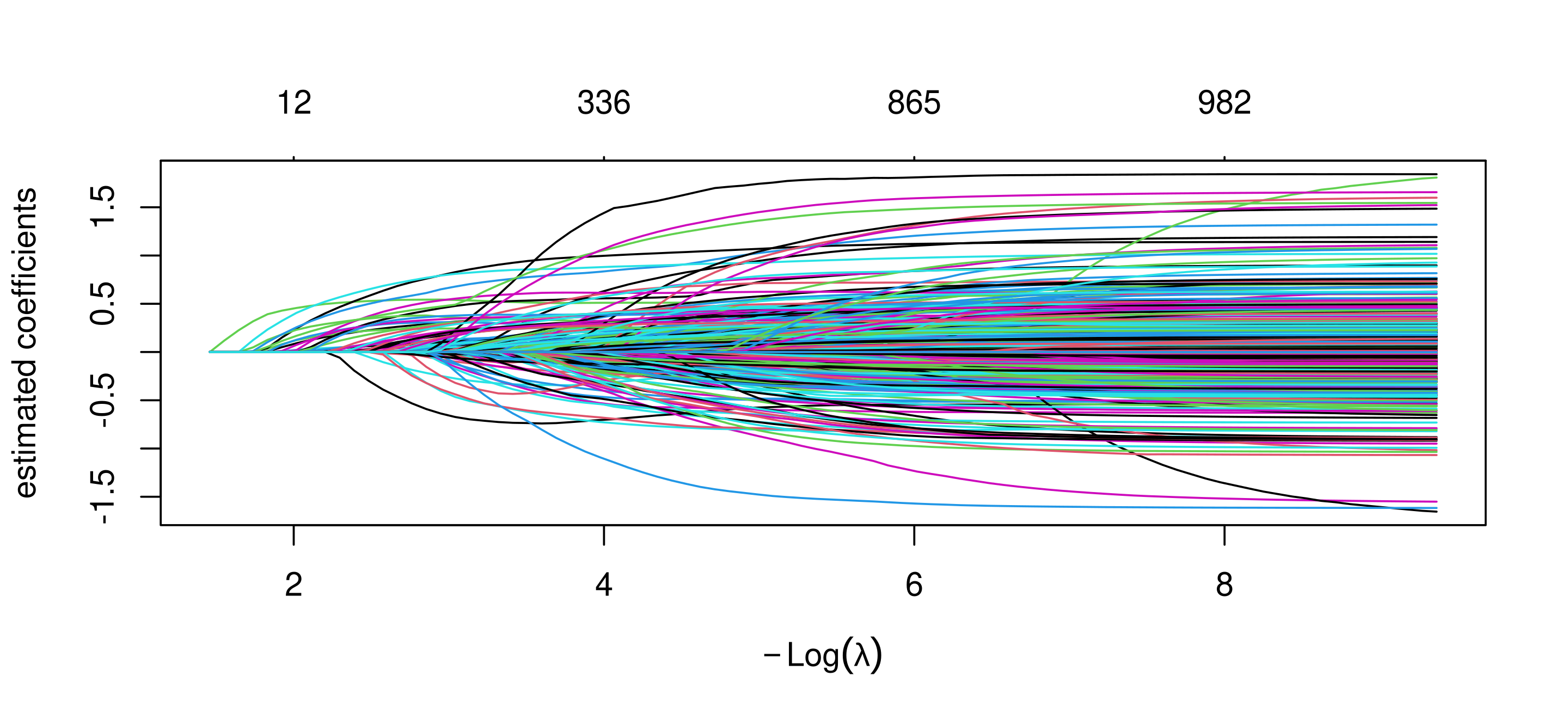
• glmnet() computed 86 lasso fits, starting at \lambda = 0.23 where every coefficient is zero and shrinking \lambda by 9% each step. It stops early once the deviance explained stops improving.
• Along the path the number of nonzero coefficients rises from 0 to 993 and the share of deviance explained from 0 to 25%.
• family = "gaussian" is least squares; "binomial" gives a penalized logit with the same syntax.

The coefficient path

plot(lasso_model, xvar = "lambda", ylab = "estimated coefficients")

Each line is one site’s coefficient as \lambda falls from right to left. The axis on top counts the nonzero coefficients. glmnet does not choose a point on this path; cross-validation does.

Choosing \lambda by cross-validation

The path is a set of candidate estimators, one per \lambda_t. Apply last lecture’s recipe:

1. Compute the regularization path \lambda_1, \dots, \lambda_T on the full data.
2. Split the data at random into K folds.
3. For each fold k, estimate \hat\beta^t for every \lambda_t on the other folds, and compute \text{dev}_{OOS}(\hat\beta^t) on fold k.
4. Average the K deviances for each \lambda_t and choose the \hat\lambda with the lowest average.
5. Refit the lasso on all the data with penalty \hat\lambda to get the final \hat\beta.

cv.glmnet() does all five steps, with K = 10 by default.

cv.glmnet() does it all

set.seed(0)
cv_lasso <- cv.glmnet(xweb, log(yspend), family = "gaussian")
plot(cv_lasso)

The fold assignment is random, so set.seed() makes the result reproducible. The loop over 10 folds and 86 penalties takes about 15 seconds.

Reading the CV plot

c(lambda.min = cv_lasso$lambda.min, lambda.1se = cv_lasso$lambda.1se)

## lambda.min lambda.1se 
## 0.02271315 0.04356178

tibble(lambda = cv_lasso$lambda, cv_error = cv_lasso$cvm, se = cv_lasso$cvsd, nonzero = cv_lasso$nzero) %>%
  filter(lambda %in% c(cv_lasso$lambda[1], cv_lasso$lambda.1se, cv_lasso$lambda.min))

## # A tibble: 3 × 4
##   lambda cv_error     se nonzero
##    <dbl>    <dbl>  <dbl>   <int>
## 1 0.232      2.78 0.0357       0
## 2 0.0436     2.51 0.0454     100
## 3 0.0227     2.47 0.0484     236

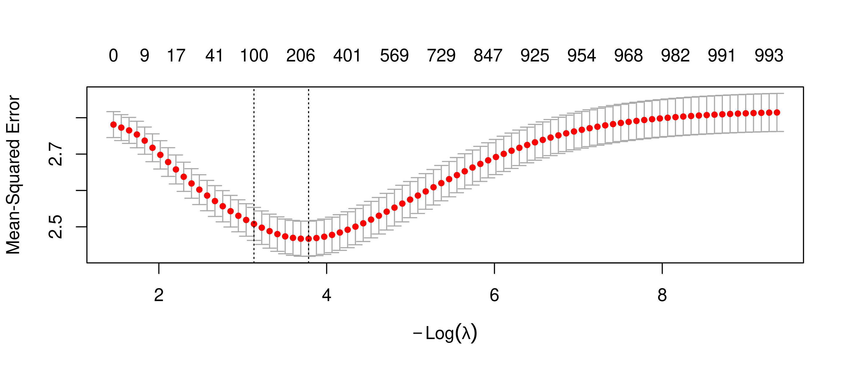
• Each point is the average out-of-sample mean squared error over the 10 folds, with plus or minus one standard error across folds.
• lambda.min (left dotted line) minimizes the CV error: 236 sites, error 2.47 against 2.78 for the intercept-only model at the top of the path, a CV R^2 of about 0.11.
• lambda.1se (right dotted line) is the largest \lambda within one standard error of the minimum: 100 sites, error 2.51.

Coefficients at the chosen \lambda

b_min <- coef(cv_lasso, s = "lambda.min")          # a sparse 1001 x 1 matrix: intercept + 1,000 sites
coefs <- tibble(site = rownames(b_min)[-1], coefficient = as.vector(b_min)[-1]) %>%
  filter(coefficient != 0)
bind_cols(coefs %>% slice_max(coefficient, n = 4), coefs %>% slice_min(coefficient, n = 4)) %>%
  knitr::kable(digits = 2, col.names = c("site", "coefficient", "site", "coefficient"))

site	coefficient	site	coefficient
shopyourbargain.com	1.25	cursormania.com	-0.96
victoriassecret.com	0.98	coolsavings.com	-0.73
bizrate.com-o01	0.96	tickle.com	-0.69
atomz.com	0.92	limewire.com	-0.65

• 236 of the 1,000 coefficients are nonzero: bargain and retail sites positive, cursor downloads and coupon sites negative.
• Coefficients are per percentage point of browsing share, and most shares are far below one point. Predictive associations, not causal effects.

Predict for new households

predict(cv_lasso, newx = xweb[1:3, ], s = "lambda.min")

##   lambda.min
## 1   5.695805
## 2   9.545932
## 3   6.064591

log(yspend[1:3])

## [1] 6.049733 7.755767 5.631212

• predict() on a cv.glmnet object takes a design matrix with the same 1,000 columns and the penalty to use. s = "lambda.1se" would use the sparser fit.
• The predictions are on the log scale, like the outcome. Household 2 is predicted to spend far more than it did; a CV R^2 of 0.11 means most of the variation in spending is not explained by where people browse.

Does it beat OLS out of sample?

set.seed(0)
n <- length(yspend); ly <- log(yspend)
test <- sample.int(n, size = round(0.2 * n)); train <- setdiff(1:n, test)   # 2,000 held out
r2 <- function(y, pred, ybar) 1 - sum((y - pred)^2) / sum((y - ybar)^2)
X_dense <- cbind(1, as.matrix(xweb))
b_ols <- lm.fit(X_dense[train, ], ly[train])$coefficients
b_ols[is.na(b_ols)] <- 0                      # one site is never visited in the training set
set.seed(0)
cv_train <- cv.glmnet(xweb[train, ], ly[train])
c(ols_in = r2(ly[train], X_dense[train, ] %*% b_ols, mean(ly[train])),
  ols_out = r2(ly[test], X_dense[test, ] %*% b_ols, mean(ly[train])),
  lasso_out = r2(ly[test], predict(cv_train, xweb[test, ], s = "lambda.min"), mean(ly[train])),
  lasso_1se_out = r2(ly[test], predict(cv_train, xweb[test, ], s = "lambda.1se"), mean(ly[train])))

##        ols_in       ols_out     lasso_out lasso_1se_out 
##    0.28151022   -0.09739119    0.10670526    0.10046033

• OLS with 1,000 regressors on 8,000 observations fits the training sample best and predicts the held-out households worse than their training-sample mean.
• The lasso’s out-of-sample R^2 matches its CV estimate, which is what CV is for.

Checkpoint: the spending lasso

1. Why fit the model to \log(\text{spend}) rather than to spending in dollars?
2. cv.glmnet() reports lambda.min with 236 sites and lambda.1se with 100. A marketing team can only track 100 sites. Which fit should it use, and what does it give up?
3. Suppose you add the 1,000 squared visit shares as extra columns. What happens to the path’s starting point, and how would you choose among the 2,000 regressors?

Answers: spending is skewed by a factor of 400,000 and the log makes the errors comparable across households; lambda.1se, giving up about 0.04 in CV error, less than one standard error; the first lambda is still the smallest penalty that zeros everything, which may change, and cv.glmnet handles 2,000 columns exactly as it handled 1,000.

Practical details

---

Folds, the one-standard-error rule, factors and standardization

How many folds?

• cv.glmnet(..., nfolds = K) sets the number of folds. The default is K = 10.
• The standard error reported for each \lambda_t is SD_{OOS}(\hat\beta^t)/\sqrt{K}: the sample standard deviation of the K fold deviances divided by \sqrt{K}, like the standard error of a sample mean. These are the bars on the CV plot.
• Wide bars that overlap across many \lambda’s mean the location of the minimum is uncertain.
• More folds mean more fits, training sets closer to the full sample, and more fold estimates to average. But each fold estimate is noisier when the folds are small, so the standard error does not shrink mechanically with K.
• K = 5 or K = 10 is the usual compromise. Leave-one-out means n fits and is rarely worth it here.

Five, ten or twenty folds on the spending data

fold_choice <- function(K) {
  set.seed(0)
  cv_k <- cv.glmnet(xweb, log(yspend), nfolds = K)
  i <- which(cv_k$lambda == cv_k$lambda.min)
  tibble(K = K, lambda.min = cv_k$lambda.min, cv_error = cv_k$cvm[i],
         se = cv_k$cvsd[i], nonzero = cv_k$nzero[i])
}
map_dfr(c(5, 10, 20), fold_choice) %>% knitr::kable(digits = 4)

K	lambda.min	cv_error	se	nonzero
5	0.0249	2.4799	0.0324	206
10	0.0227	2.4672	0.0484	236
20	0.0227	2.4716	0.0447	236

• Ten and twenty folds agree on \lambda and on 236 sites; five folds choose a slightly larger \lambda and 206 sites. The 20-fold run takes twice as long as the 10-fold one for the same answer.

The one-standard-error rule

• The standard errors are also used to choose \lambda. Any \lambda whose CV error is within one standard error of the minimum is statistically as good as the best.
• Among those, prefer the largest \lambda: it has the fewest nonzero coefficients, so a prediction needs less data to collect and the model is easier to read.
• cv.glmnet() returns this choice as lambda.1se, and coef() and predict() accept s = "lambda.1se".

tibble(choice = c("lambda.min", "lambda.1se"),
       lambda = c(cv_lasso$lambda.min, cv_lasso$lambda.1se),
       nonzero = c(sum(coef(cv_lasso, s = "lambda.min")[-1] != 0),
                   sum(coef(cv_lasso, s = "lambda.1se")[-1] != 0)))

## # A tibble: 2 × 3
##   choice     lambda nonzero
##   <chr>       <dbl>   <int>
## 1 lambda.min 0.0227     236
## 2 lambda.1se 0.0436     100

On the spending data the rule trades 136 sites for a CV error 0.04 higher, less than one standard error (0.05).

Regularization breaks reparameterization invariance

Without regularization, many estimators are invariant to common reparameterizations:

• Rescale a regressor (miles to yards) and the OLS coefficient rescales accordingly; fitted values and the economic meaning are unchanged.
• Drop a different dummy from a factor and the OLS fit is the same; only the interpretation of the coefficients shifts.

With a penalty on the size of the coefficients, neither holds any more. The penalty is attached to the numbers \beta_j, and the numbers depend on how the regressors are written down.

Two practical fixes follow: keep every level of a factor, and standardize the covariates.

Categorical variables: keep every level

• OLS with a factor drops one dummy, the reference level, to avoid perfect collinearity with the intercept.
• Under regularization, shrinking a coefficient to zero means pushing that level toward the reference level. Change the reference level and the results change.
• The fix: keep all the dummies plus an intercept. Every level is then shrunk toward a shared intercept, which treats the levels symmetrically.
• OLS could not do this (perfect collinearity), but the penalty makes the solution unique even with collinear columns.
• Omitting the intercept instead would shrink every level toward zero, which rarely makes sense: why should the orange juice intercepts be near zero?

In R, model.matrix(~ brand + price - 1) keeps all the brand dummies; glmnet() then adds its own intercept. (gamlr has a helper, naref(), for the same purpose.)

Orange juice: two codings, two answers

oj <- read.csv("data/oj.csv"); oj$brand <- factor(oj$brand)
x_all <- model.matrix(~ brand + price - 1, data = oj)     # three brand dummies and price
x_ref <- model.matrix(~ brand + price, data = oj)[, -1]   # dominicks dropped, as lm() would
fit_all <- glmnet(x_all, log(oj$sales)); fit_ref <- glmnet(x_ref, log(oj$sales))
b_all <- coef(fit_all, s = 0.1); b_ref <- coef(fit_ref, s = 0.1)
tab <- cbind(all_levels = as.vector(b_all), reference_level = c(b_ref[1], 0, b_ref[-1]))
rownames(tab) <- rownames(b_all)
round(tab, 3)

##                  all_levels reference_level
## (Intercept)          10.906          10.574
## branddominicks       -0.282           0.000
## brandminute.maid      0.000           0.000
## brandtropicana        0.227           0.283
## price                -0.754          -0.657

• Same data, same \lambda = 0.1, different answers. With every level kept, Minute Maid’s coefficient is zero and the other two brands sit symmetrically around the shared intercept.
• With Dominicks as the reference, “zero” means equal to Dominicks: Minute Maid is pulled onto Dominicks and Tropicana’s gap is larger. The fitted values differ too.
• OLS gives identical fits either way: intercept 11.49 with brand effects 0.72 and 1.45.

Standardize the covariates

• With OLS the scale of a covariate does not matter: convert miles to yards and the coefficient adjusts so that X_1\beta_1 is unchanged.
• The lasso penalizes every coefficient by the same \lambda, so covariates on different scales are penalized differently: X_1\beta_1 = (2X_1)(\beta_1/2), and the penalty on \beta_1/2 is half the penalty on \beta_1. Doubling X_1 makes it cheaper to include.
• To penalize every covariate the same, standardize the penalty: \lambda \sum_{k=1}^d \text{sd}(X_k)\,|\beta_k|. Doubling X_1 now doubles \text{sd}(X_1) and the penalty is unchanged.
• glmnet() standardizes by default (standardize = TRUE) and reports the coefficients on the original scale. Turn it off only when the regressors are already on a common scale and you mean to penalize them unequally, for example indicators.

Dollars or cents?

x_cents <- x_all; x_cents[, "price"] <- 100 * x_all[, "price"]      # price in cents instead of dollars
coef_at <- function(x, standardize)
  as.vector(coef(glmnet(x, log(oj$sales), standardize = standardize), s = 0.05))
rbind(standardized_dollars = coef_at(x_all, TRUE),  standardized_cents = coef_at(x_cents, TRUE),
      raw_dollars = coef_at(x_all, FALSE),          raw_cents = coef_at(x_cents, FALSE)) %>%
  `colnames<-`(c("intercept", colnames(x_all))) %>% round(4)

##                      intercept branddominicks brandminute.maid brandtropicana   price
## standardized_dollars   11.5543        -0.4987                0         0.4797 -1.0427
## standardized_cents     11.5543        -0.4987                0         0.4797 -0.0104
## raw_dollars            11.0327        -0.3018                0         0.2540 -0.8100
## raw_cents              10.7087         0.0000                0         0.0000 -0.0068

• Standardized: the two codings give the same model; the price coefficient is simply 100 times smaller per cent than per dollar.
• Unstandardized: measuring price in cents makes its coefficient tiny and cheap to keep, so at the same \lambda the lasso drops all three brand dummies and keeps only price. The selected model depends on the units.

Checkpoint: practical details

1. A colleague fits a lasso with brand coded with Tropicana as the reference level and finds that Minute Maid “does not matter”. What is the problem?
2. Income is measured in dollars and age in years. Without standardization, which is penalized more heavily per unit of economic effect?
3. Why is lambda.1se always at least as large as lambda.min?

Answers: zero means equal to Tropicana, not unimportant, and the result depends on the arbitrary reference; income, since its coefficient per dollar is tiny and the penalty acts on the coefficient’s size, so a large-scale variable is cheap and a small-scale one dear, which is backwards from the colleague’s intuition, so standardize; by definition it is the largest lambda within one standard error of the minimum, and lambda.min itself qualifies.

Beyond the lasso

---

The elastic net for correlated regressors, the group lasso for grouped ones

Correlated regressors trouble the lasso

Suppose two columns are identical, X_j = X_k, and the lasso solution has \hat\beta_j > 0. Then

• \hat\beta_k \ge 0 too (the signs agree), and
• moving the pair to (0, \hat\beta_j + \hat\beta_k) leaves the fit and the penalty unchanged: the solution is not unique, and the lasso picks one of the twins arbitrarily.

With highly (not perfectly) correlated regressors the choice between them is unstable from sample to sample.

• Ridge behaves differently: it shrinks correlated regressors’ coefficients toward each other, and twins get identical coefficients.
• Ridge, however, does not select. We want both: stability on correlated groups and exact zeros.

Bridge penalties and the elastic net

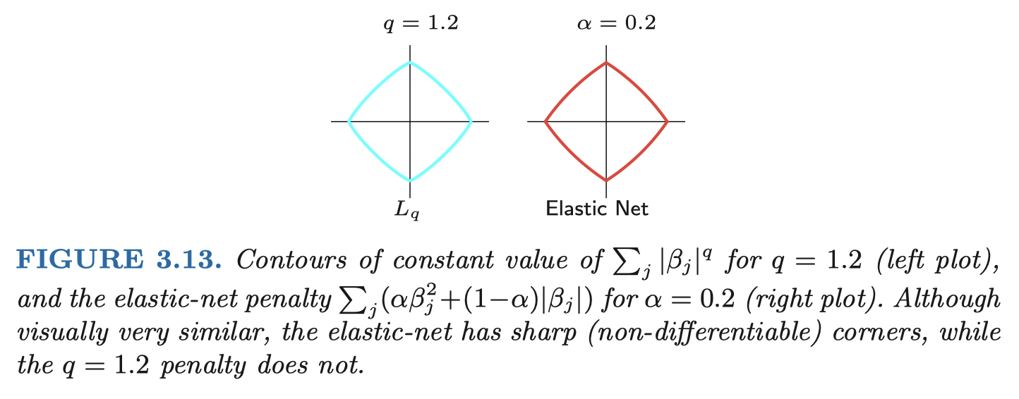
Lasso and ridge are the q = 1 and q = 2 members of the bridge family \lambda \sum_j |\beta_j|^q:

• q between 1 and 2 compromises between the two, but the computation is awkward and the region has no corners for q > 1.
• The elastic net mixes the two penalties instead of the two exponents: \min_{\beta} \left\{ \tfrac{1}{2}\lVert y - X\beta \rVert^2 + \lambda\big[(1 - \alpha)\lVert\beta\rVert_1 + \alpha\lVert\beta\rVert_2^2\big] \right\}, \qquad \alpha \in [0, 1], with \alpha = 0 the lasso and \alpha = 1 ridge, in the notation of the notes.

[Sources] - Frank and Friedman (1993), Technometrics, for the bridge; Zou and Hastie (2005), JRSS-B 67, 301-320, for the elastic net. - The figure is figure 2.6 of Hastie, Tibshirani and Wainwright (2015), Statistical Learning with Sparsity.

What the elastic net buys

Elastic net with mixing 0.2 (left) and the bridge ball with q = 1.2 (right). The elastic net keeps its corners.

• Uniqueness: any ridge weight makes the objective strongly convex, so the solution is unique.
• Selection: the corners survive, so coefficients are still set exactly to zero. More than n regressors can be kept, which the lasso cannot do.
• Grouping: for two regressors with coefficients of the same sign, |\hat\beta_j - \hat\beta_k| \le \frac{\lVert X_j - X_k \rVert_2}{2\lambda\alpha}\,\lVert y \rVert_2, so similar columns get similar coefficients and twins get equal ones (proof in the appendix).

[Sources] - The figure is figure 3.13 of Hastie, Tibshirani and Friedman (2009).

The elastic net in glmnet

glmnet‘s alpha is the weight on the lasso part: alpha = 1 (the default) is the lasso and alpha = 0 is ridge. The notes’ \alpha is one minus glmnet’s.

alpha_choice <- function(a) {
  set.seed(0); cv_a <- cv.glmnet(xweb, log(yspend), alpha = a)
  i <- which(cv_a$lambda == cv_a$lambda.min)
  tibble(alpha = a, lambda.min = cv_a$lambda.min, cv_error = cv_a$cvm[i], se = cv_a$cvsd[i], nonzero = cv_a$nzero[i])
}
map_dfr(c(1, 0.5, 0), alpha_choice) %>% knitr::kable(digits = 4)

alpha	lambda.min	cv_error	se	nonzero
1.0	0.0227	2.4672	0.0484	236
0.5	0.0454	2.4664	0.0478	235
0.0	2.2191	2.4780	0.0311	1000

Same folds, three mixes: the CV errors differ by a fraction of a standard error, ridge keeps all 1,000 sites, the other two about 236. cv.glmnet() does not search over alpha; try a few values and compare.

glmnet’s objective is (1/2n) RSS + lambda [ (1 - alpha)/2 ||beta||_2^2 + alpha ||beta||_1 ], so the ridge term carries a factor one half. On these data the elastic net buys stability at no cost in CV error; alpha is a second tuning parameter chosen by comparing CV errors across a few values.

The group lasso: zero out groups together

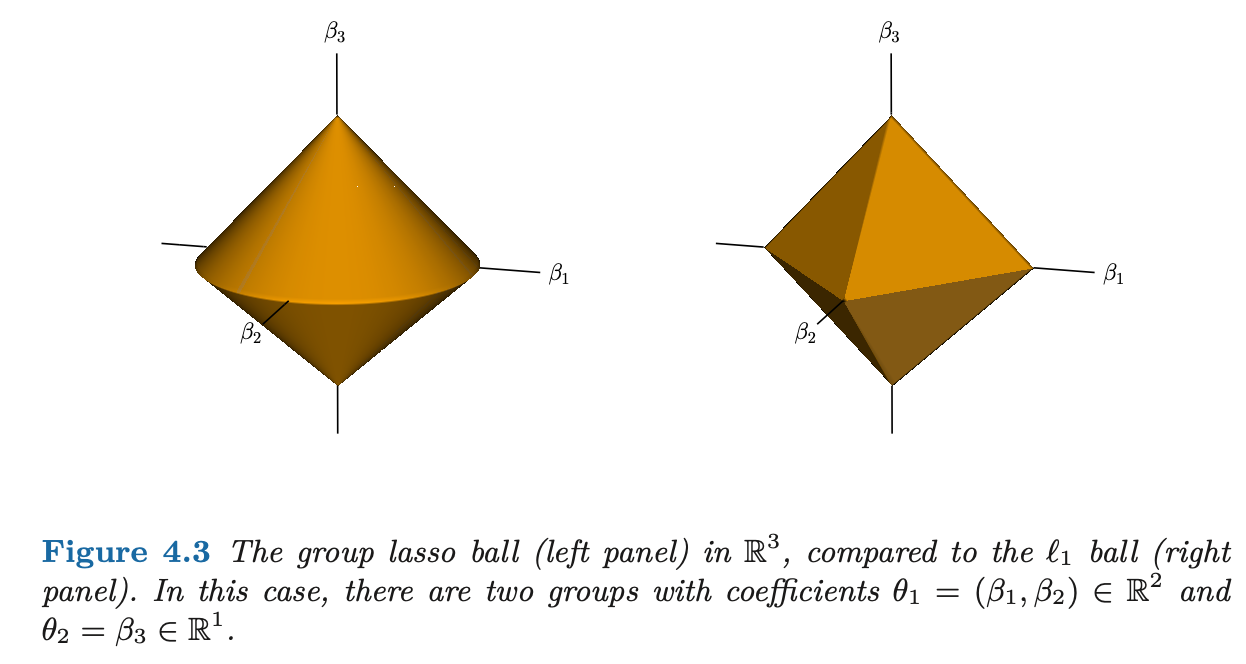
Sometimes regressors come in predefined groups and we want a whole group in or out:

• A categorical variable with K levels is K dummy columns. Dropping the variable means dropping all K at once.
• In an additive model f(x) = \sum_j f_j(x_j) with each f_j expanded in basis functions, f_j(x_j) = \sum_{\ell=1}^{q_j} \beta_{j\ell}\,\psi_{j\ell}(x_j), removing regressor j means zeroing (\beta_{j1}, \dots, \beta_{jq_j}) together.
• In multitask regression of m outcomes on the same X, \min_B \tfrac12 \lVert Y - XB \rVert_F^2 splits into m separate regressions. If X_j is irrelevant to every outcome we want its whole row B_{j\cdot} to be zero.

The lasso penalizes each coefficient separately and knows nothing about the groups.

The group lasso penalty

Partition \{1, \dots, p\} into groups g_1, \dots, g_L. The group lasso solves

\min_\beta\ \tfrac12 \lVert y - X\beta \rVert^2 + \lambda \sum_{\ell=1}^L w_\ell\, \lVert \beta_{g_\ell} \rVert_2,

with known weights w_\ell, usually w_\ell = \sqrt{|g_\ell|} to account for group size.

• The key is \lVert \beta_{g_\ell} \rVert_2, not squared. For a group of size one it is |\beta_j| and the group lasso is the lasso.
• For a group of size two, \sqrt{\beta_1^2 + \beta_2^2} is a cone with a kink at the origin, so the whole group can sit at exactly zero.
• The constraint region is round within a group (ridge-like) and spiky across groups (lasso-like).

[Sources] - Yuan and Lin (2006), Model selection and estimation in regression with grouped variables, JRSS-B 68, 49-67. - The figure is figure 4.3 of Hastie, Tibshirani and Wainwright (2015).

Groupwise soft-thresholding

For an orthonormal design the group lasso has the same closed form as the lasso, applied to groups:

\hat\beta_{g_\ell} = \left(1 - \frac{\lambda w_\ell}{\lVert \hat\beta^{\,\text{OLS}}_{g_\ell} \rVert_2}\right)_+ \hat\beta^{\,\text{OLS}}_{g_\ell}, \qquad (a)_+ = \max\{a, 0\}.

• If the group’s OLS coefficients have norm above \lambda w_\ell, the vector is shrunk toward zero by \lambda w_\ell in length, with its direction kept.
• If the norm is at most \lambda w_\ell, the entire group is set to zero.
• Larger groups have larger norms by construction, which is why the weight w_\ell = \sqrt{|g_\ell|} is the usual choice.

Back to multitask learning: penalizing \sum_j \lVert B_{j\cdot} \rVert_2 ties the m regressions together and selects regressors that matter for all outcomes at once. Groups that overlap, as genes in biological pathways do, need more care (appendix).

Packages: grpreg and gglasso fit the group lasso in R; neither is installed in this environment, so the deck stays conceptual. The closed form is the proximal operator of the penalty, derived in the appendix.

Checkpoint: beyond the lasso

1. Two sites are visited by exactly the same households in the same proportions. What does the lasso do with them, and what does the elastic net do?
2. A regression has a 12-level factor. Why might you prefer the group lasso to the lasso for deciding whether the factor matters?
3. With group weights w_\ell = 1 for every group, which groups would the group lasso tend to keep?

Answers: the lasso picks one arbitrarily or splits the coefficient between them in a non-unique way, the elastic net gives them equal coefficients; the lasso could keep three levels and drop nine, which is neither “in” nor “out”, while the group lasso decides for the whole factor; large groups, because their coefficient vectors have larger norms and clear the threshold more easily.

Regularization in one page

A penalty turns a combinatorial search into a path. Instead of 2^d subsets, minimize deviance plus \lambda \sum_j c(\beta_j) and let \lambda index the candidates from the empty model to OLS.

Lasso selects, ridge only shrinks. The \ell_1 corners put coefficients exactly at zero; the \ell_2 disc does not. Both trade bias for variance.

glmnet() fits the path, cv.glmnet() picks the point. lambda.min for the best estimated error, lambda.1se for the sparsest model that is statistically as good.

Regularization is not invariant to how the regressors are written. Keep every level of a factor and standardize the covariates, which glmnet does by default.

Elastic net and group lasso extend the idea. Mix in ridge for correlated regressors; penalize group norms to select whole groups.

Reading and data sources

• James, Witten, Hastie and Tibshirani, An Introduction to Statistical Learning, chapter 6: ridge, lasso and their geometry.
• Hastie, Tibshirani and Friedman, The Elements of Statistical Learning, sections 3.4 and 3.8: shrinkage methods, LARS and related paths.
• Hastie, Tibshirani and Wainwright, Statistical Learning with Sparsity (2015): the lasso, its uniqueness theory, the elastic net and the group lasso.
• Tibshirani (1996), the lasso; Zou and Hastie (2005), the elastic net; Yuan and Lin (2006), the group lasso; Efron, Hastie, Johnstone and Tibshirani (2004), least angle regression; Tibshirani (2013), the lasso problem and uniqueness.
• glmnet vignette: the package’s syntax, families and cross-validation; Boyd and Vandenberghe, Convex Optimization.
• Taddy, Business Data Science (2019), chapter 3: the browsing data and the spending application.

Additional derivations and code

---

Optional material for reference and practice

Ridge regression in closed form

Ridge minimizes \lVert y - X\beta \rVert^2 + \lambda \lVert \beta \rVert^2 over \beta \in \mathbb{R}^p. The objective is differentiable, so the first-order condition is

-2X'(y - X\hat\beta_\lambda) + 2\lambda\hat\beta_\lambda = 0 \quad\Longleftrightarrow\quad \hat\beta_\lambda = (X'X + \lambda I_p)^{-1} X'y.

• Every eigenvalue of X'X + \lambda I_p is at least \lambda > 0, so the inverse exists whatever X is: ridge always has a unique minimizer, even with p > n or identical columns.
• As \lambda \downarrow 0 the solution tends to the minimum-norm least squares solution X^+ y, which is OLS when X'X is invertible.
• With y \sim N(X\beta, \sigma^2 I): \mathbf{E}\hat\beta_\lambda = (X'X + \lambda I)^{-1}X'X\beta \ne \beta for \lambda > 0 (biased), and \text{Cov}(\hat\beta_\lambda) = \sigma^2 (X'X + \lambda I)^{-1} X'X (X'X + \lambda I)^{-1} is smaller than the OLS covariance \sigma^2 (X'X)^{-1}.

Ridge: the bias-variance trade-off in the orthonormal case

With X'X = I_p, \hat\beta_\lambda = X'y/(1 + \lambda), so

\mathbf{E}\hat\beta_\lambda = \frac{\beta}{1 + \lambda}, \qquad \text{Cov}(\hat\beta_\lambda) = \frac{\sigma^2}{(1 + \lambda)^2} I_p,

and the mean squared error \mathbf{E}\lVert \hat\beta_\lambda - \beta \rVert^2 splits into total variance plus squared bias:

\text{MSE}(\lambda) = \frac{\sigma^2 p}{(1 + \lambda)^2} + \left(\frac{1}{1 + \lambda} - 1\right)^2 \lVert\beta\rVert^2 = \frac{\sigma^2 p + \lambda^2 \lVert\beta\rVert^2}{(1 + \lambda)^2}.

Setting the derivative to zero gives the MSE-optimal penalty \lambda^\ast = \frac{\sigma^2 p}{\lVert\beta\rVert^2} = \frac{1}{\text{signal-to-noise ratio}}.

High signal-to-noise: \lambda^\ast \approx 0, almost OLS. Low signal-to-noise: heavy shrinkage. Cross-validation estimates this trade-off without knowing \sigma^2 or \beta.

The lasso’s optimality conditions

The lasso objective f(\beta) = \tfrac12 \lVert y - X\beta \rVert^2 + \lambda \lVert\beta\rVert_1 is convex but not differentiable at zero. Replace the gradient by the subdifferential, the set of slopes of lines that support f from below. For the absolute value,

\partial |\beta_j| = \begin{cases} \{\text{sgn}(\beta_j)\} & \beta_j \ne 0, \\ [-1, 1] & \beta_j = 0, \end{cases}

and \hat\beta minimizes f if and only if 0 \in \partial f(\hat\beta). Written out, the KKT conditions are

X'(y - X\hat\beta_\lambda) = \lambda s, \qquad s_j = \text{sgn}(\hat\beta_{\lambda,j}) \text{ if } \hat\beta_{\lambda,j} \ne 0, \quad s_j \in [-1, 1] \text{ if } \hat\beta_{\lambda,j} = 0.

• \lambda = 0 recovers the OLS normal equations X'(y - X\hat\beta) = 0.
• |X_j'(y - X\hat\beta_\lambda)| < \lambda implies \hat\beta_{\lambda,j} = 0: a regressor enters only when its correlation with the residual reaches \lambda. Hence \lambda_{\max} = \lVert X'y \rVert_\infty zeros everything.
• Between the events where a coefficient enters or leaves, the conditions are linear, so the path is piecewise linear in \lambda.

Soft-thresholding follows directly: with X’X = I the condition for coefficient j reads b_j - beta_j = lambda s_j, whose solution is sgn(b_j)(|b_j| - lambda)_+ where b_j = X_j’y. The appendix slide on the subgradient figure in the notes is replaced by this algebra.

When is the lasso solution unique?

The solution \hat\beta_\lambda need not be unique (twin columns), but several things always are:

• The fit X\hat\beta_\lambda: write the problem as minimizing \tfrac12 \lVert y - u \rVert^2 + \lambda\, h(u) with h(u) = \min\{\lVert\beta\rVert_1 : X\beta = u\} convex in u. The objective is strictly convex in u, so \hat u = X\hat\beta_\lambda is unique.
• The penalty value \lVert \hat\beta_\lambda \rVert_1 and the subgradient \hat s = X'(y - \hat u)/\lambda, since both are functions of \hat u.
• The sign pattern is consistent across solutions: \hat\beta_{\lambda,j} > 0 forces \hat s_j = 1 and hence \tilde\beta_{\lambda,j} \ge 0 in any other solution.

The active set \mathcal{A}_\lambda = \{j : \hat\beta_{\lambda,j} \ne 0\} can differ across solutions, but every active set lies in the equicorrelation set \mathcal{E}_\lambda = \{j : |X_j'(y - X\hat\beta_\lambda)| = \lambda\}, the largest possible active set, which is the one LARS produces. Some solution has at most \min\{n, p\} nonzero coefficients.

[Sources] - Tibshirani (2013), The lasso problem and uniqueness, Electronic Journal of Statistics 7, 1456-1490.

Least angle regression

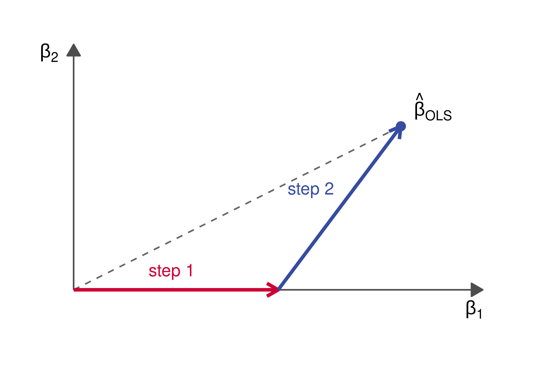
With standardized regressors, X_j'(y - X\beta) is the correlation between X_j and the residual. LARS (Efron, Hastie, Johnstone and Tibshirani 2004) follows how these correlations change as \lambda falls from \lambda_{\max}:

1. Start with r = y - \bar y and \beta = 0. Find the regressor X_j most correlated with r.
2. Move \beta_j toward its least squares value until another regressor X_k is as correlated with the residual as X_j.
3. Move \beta_j and \beta_k jointly in the direction of their joint least squares fit until a third regressor catches up, and so on until all \min\{n - 1, p\} have entered.

Two regressors: X_1 enters first, then X_2 joins and the path turns toward OLS.

From LARS to the lasso path

• Like forward selection, LARS is greedy and adds one variable at a time, but it enters only “as much” of a variable as its correlation with the residual deserves.
• By construction the coefficients are piecewise linear in the step length, and the step length has a closed form, so the whole path costs about as much as one least squares fit.
• Lasso modification. The KKT sign condition says an active coefficient must share the sign of its correlation with the residual. If a coefficient hits zero along the LARS path, drop its variable from the active set and recompute the joint least squares direction. The modified algorithm computes the exact lasso path.
• The lars package implements both; its diabetes example in the notes shows the two paths side by side, identical until a coefficient crosses zero.

[Sources] - Efron, Hastie, Johnstone and Tibshirani (2004), Least angle regression, Annals of Statistics 32, 407-499; Hastie, Tibshirani and Friedman (2009), section 3.4.4 and exercise 3.25 for the step length. The notes animate this picture with gganimate and show the lars package’s diabetes example; neither package is installed here.

The elastic net’s grouping bound

Take \hat\beta_j \hat\beta_k > 0 and write \hat r = y - X\hat\beta. The KKT conditions for the two coefficients are

-X_j'\hat r + \lambda(1 - \alpha) s_j + 2\lambda\alpha\hat\beta_j = 0, \qquad -X_k'\hat r + \lambda(1 - \alpha) s_k + 2\lambda\alpha\hat\beta_k = 0,

with s_j = s_k because the signs agree. Subtracting,

2\lambda\alpha\,(\hat\beta_j - \hat\beta_k) = (X_j - X_k)'\hat r \quad\Longrightarrow\quad |\hat\beta_j - \hat\beta_k| \le \frac{\lVert X_j - X_k \rVert_2\, \lVert \hat r \rVert_2}{2\lambda\alpha} \le \frac{\lVert X_j - X_k \rVert_2\, \lVert y \rVert_2}{2\lambda\alpha}

by Cauchy-Schwarz and because the minimized objective is at most its value at \beta = 0, so \tfrac12 \lVert \hat r \rVert^2 \le \tfrac12 \lVert y \rVert^2.

Identical columns give identical coefficients, and the bound tightens as the columns get closer or the ridge weight \lambda\alpha grows.

The elastic net as a lasso on augmented data

Stack p fake observations under the data:

\tfrac12 \lVert y - X\beta \rVert^2 + \lambda\big[(1 - \alpha)\lVert\beta\rVert_1 + \alpha\lVert\beta\rVert_2^2\big] = \tfrac12 \left\lVert \underbrace{\begin{pmatrix} y \\ 0_p \end{pmatrix}}_{\text{new } y} - \underbrace{\begin{pmatrix} X \\ \sqrt{2\lambda\alpha}\, I_p \end{pmatrix}}_{\text{new } X} \beta \right\rVert^2 + \underbrace{\lambda(1 - \alpha)}_{\text{new } \lambda} \lVert\beta\rVert_1 .

• The ridge part becomes \tfrac12 \lVert \sqrt{2\lambda\alpha}\,\beta \rVert^2 = \lambda\alpha\lVert\beta\rVert_2^2, so any lasso solver handles the elastic net.
• The augmented design has n + p rows and full column rank, which is where the uniqueness comes from.
• As \alpha \downarrow 0 the solution tends to the minimum-\ell_2-norm lasso solution, which is the one LARS computes.

Overlapping groups

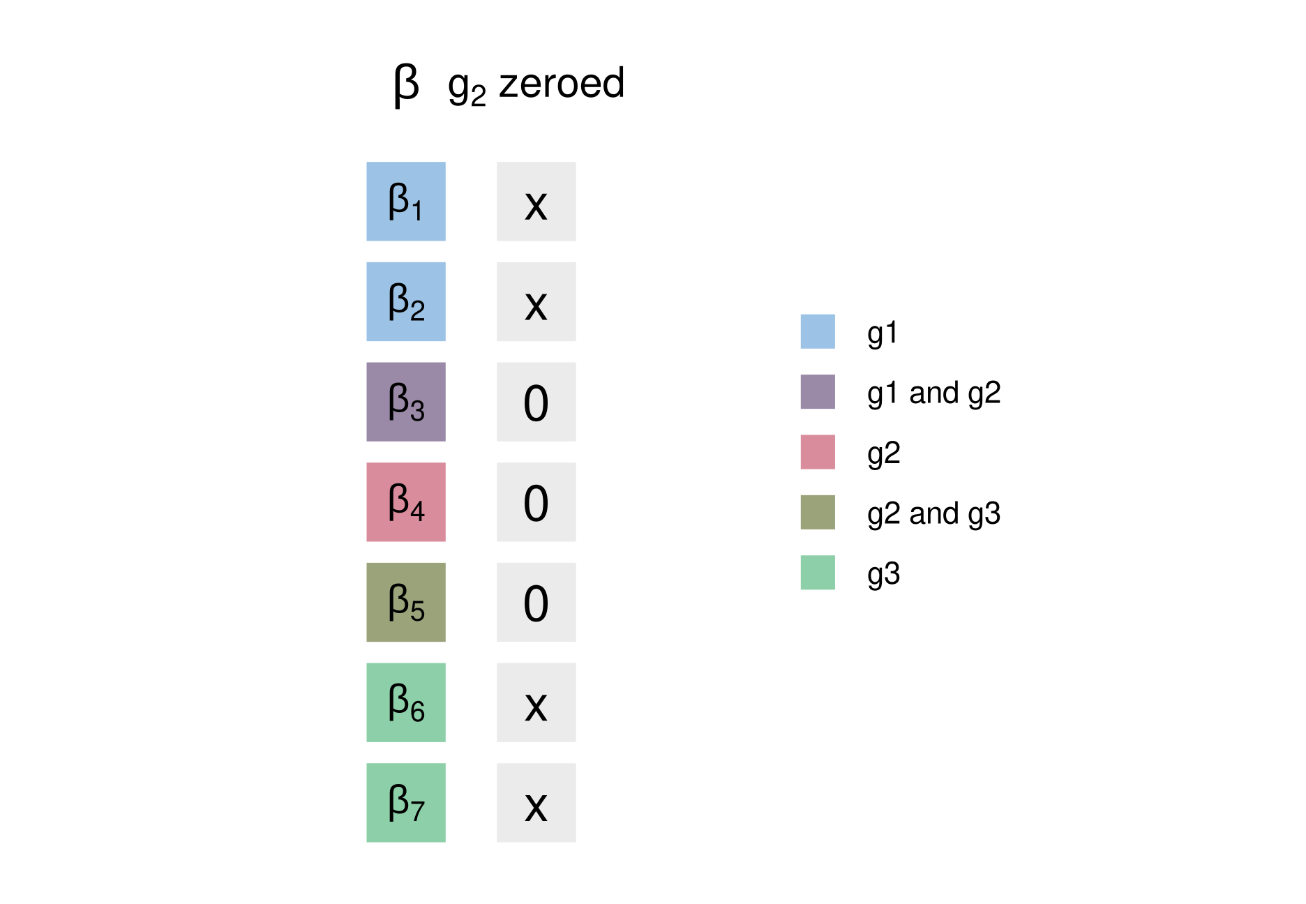
• Groups can share coefficients: genes belong to several biological pathways.
• With overlapping groups, zeroing a group zeros its whole block, so the support of \hat\beta is the complement of a union of zeroed groups, not a union of kept groups. Zeroing g_2 here also removes \beta_3 and \beta_5 from g_1 and g_3.
• The proximal operator then has no closed form. Its dual is a projection problem, \min \tfrac12 \lVert y - \sum_\ell \eta^{(\ell)} \rVert^2 subject to \lVert \eta^{(\ell)} \rVert_2 \le \lambda w_\ell and \eta^{(\ell)} zero outside g_\ell, solved by block coordinate descent; without overlap each block is a projection onto an \ell_2 ball.

[Sources] - Jenatton, Audibert and Bach (2011), Structured variable selection with sparsity-inducing norms, JMLR 12, 2777-2824. Without overlap the dual decouples by group and gives the groupwise soft-thresholding formula of the main lesson.

The latent overlapping group lasso

Obozinski, Jacob and Vert (2011) decompose \beta into one component per group,

\beta = \sum_{\ell=1}^L v^{(\ell)}, \qquad v^{(\ell)}_{g_\ell^c} = 0,

and penalize the components rather than \beta itself:

P_{\text{LOG}}(\beta) = \min_{v^{(1)}, \dots, v^{(L)}} \left\{ \sum_{\ell=1}^L \lVert v^{(\ell)} \rVert_2 \ :\ v^{(\ell)}_{g_\ell^c} = 0,\ \beta = \sum_\ell v^{(\ell)} \right\}.

• Now the support of \hat\beta is a union of groups: each kept v^{(\ell)} switches on its whole group, and overlapping coefficients are shared between components.
• P_{\text{LOG}} is convex because it is the partial minimum, over the v’s, of a function that is jointly convex in (v^{(1)}, \dots, v^{(L)}, \beta): the sum of norms plus the indicator functions of the two linear constraints.

[Sources] - Obozinski, Jacob and Vert (2011), Group lasso with overlaps: the latent group lasso approach, arXiv:1110.0413.

Soft-thresholding, verified

set.seed(1)
n_o <- 400
Q <- qr.Q(qr(matrix(rnorm(n_o * 3), n_o, 3))) * sqrt(n_o)   # orthogonal columns, sum of squares n
y_o <- as.vector(Q %*% c(2, 0.5, -1) + rnorm(n_o))
b_ols <- coef(lm(y_o ~ Q - 1))
lasso_fit <- glmnet(Q, y_o, lambda = 0.8, standardize = FALSE, intercept = FALSE)
rbind(ols = b_ols, glmnet_lasso = as.vector(coef(lasso_fit))[-1],
      soft_threshold = sign(b_ols) * pmax(abs(b_ols) - 0.8, 0))

##                      Q1        Q2         Q3
## ols            2.022251 0.4010225 -1.0317922
## glmnet_lasso   1.222251 0.0000000 -0.2317922
## soft_threshold 1.222251 0.0000000 -0.2317922

• glmnet minimizes \tfrac{1}{2n}\lVert y - X\beta \rVert^2 + \lambda\lVert\beta\rVert_1, so with X'X = nI the lasso coefficient is exactly \text{sgn}(\hat\beta_j)(|\hat\beta_j| - \lambda)_+: the middle coefficient, 0.4 under OLS, is set to zero.
• Ridge in the same scaling solves (X'X/n + \lambda I)^{-1}X'y/n = \hat\beta/(1 + \lambda); glmnet’s ridge path uses a different internal normalization, so compare it with the closed form of the ridge appendix slide rather than with this formula.

Install the required packages

Run once in your R environment if needed:

install.packages(c("tidyverse", "Matrix", "glmnet"))

Data files, all read from lectures/data/:

• browser-totalspend.csv, browser-domains.csv and browser-sites.txt, the household browsing panel;
• oj.csv, the orange juice data from the linear regression lecture.

The notes additionally use gamlr, lars (the diabetes example), gganimate and rgl for illustrations; none is needed to run this deck.

Return to the question

A thousand regressors and ten thousand households: OLS fit the sample and failed the test. The lasso path, with \lambda chosen by cross-validation, kept a few hundred sites and predicted better. Regularization is how we make rich models honest.

Return to the main takeaway