ECON 4370 / 6370 Computing for Economics

Lecture 11: Fundamental Concepts in Machine Learning

Zhan Gao

08 October 2026

Same data, two models

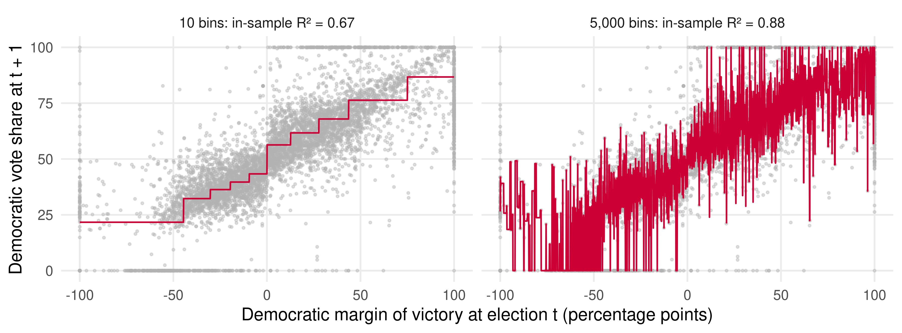
Both curves are averages of the next election’s vote share within bins of today’s margin. The right one fits this sample far better. Which one would you use to predict next year’s elections?

In-sample fit is not the goal. A prediction model is judged on data it has never seen.

Let students vote before moving on. The right panel reproduces the raw outcomes: almost every bin holds one election, so the “prediction” is one noisy observation. Lecture 9 previewed the idea with the hotel reviews, where the AUC was reported on 40,000 held-out reviews.

Today’s route

1. Overfitting: why in-sample fit cannot choose a model.
2. Out-of-sample fit and cross-validation: estimating prediction error with the sample we have.
3. The bias-variance trade-off: why cross-validation works and why complexity cuts both ways.
4. Information criteria: a formula that substitutes for the cross-validation loop.

Additional derivations and code follow the main lesson.

Connect to the last two lectures: deviance and R-squared were in-sample measures, and the hotel example already reported an out-of-sample AUC. The next lecture (regularized regression) uses K-fold CV and AICc to choose the lasso penalty, so the recipe built here is used immediately.

Packages and data

Run the examples from the lectures/ directory.

library(tidyverse)
library(RDHonest)   # provides the lee08 data set

Object	Role
lee08 (from RDHonest)	6,558 U.S. House elections: the Democratic margin of victory and the Democratic vote share at the next election

Everything else in this lecture is simulated inside the deck, so no file is read from data/.

[Sources] - https://cran.r-project.org/package=RDHonest - Lee (2008), Journal of Econometrics 142, 675-697. The data set is documented in ?lee08 and comes from the Mostly Harmless Econometrics data archive. Installation is in the appendix.

Overfitting

---

Fitting this sample is not the same as predicting the next one

Fit so far has been in-sample

• For linear and logistic regression we measured fit by the deviance and R^2 = 1 - \text{deviance}/\text{null deviance}.
• Both use the same Y_1, \dots, Y_n to fit the model and to judge it. They measure in-sample fit: how well the model fits this particular sample.
• The purpose of a prediction model is different: predict Y for new observations, which is out-of-sample prediction.
• Given several candidate models, which one will predict new data best? Picking the highest R^2 is the wrong answer.

Fitting past data too well usually makes a model predict new data worse. This is overfitting, and avoiding it is one of the main concerns of machine learning.

Every model is signal plus noise

Y_i = \underbrace{X_i'\beta}_{\text{signal}} + \underbrace{\varepsilon_i}_{\text{noise}}, \qquad \mathbf{E}[\varepsilon_i \mid X_i] = 0.

• A prediction for a new X should reproduce the signal: X'\hat\beta for the regression model.
• The noise is specific to each observation. It is mean zero and it does not repeat in the next draw.
• A model fitted too closely to the sample ends up tracking \varepsilon_i as if it were signal. That part of the fit predicts nothing.
• Chasing noise can produce predictions that are worse than the no-covariate prediction \bar Y.

R^2 rewards complexity even when there is no signal

set.seed(1)
n_noise <- 50
y_noise <- rnorm(n_noise)         # pure noise
X_noise <- matrix(rnorm(n_noise * 49), n_noise, 49)
r2 <- sapply(1:49, function(k)    # k noise regressors
  summary(lm(y_noise ~ X_noise[, 1:k]))$r.squared)
round(r2[c(1, 10, 25, 49)], 2)

## [1] 0.00 0.33 0.68 1.00

• R^2 never falls when a regressor is added, whatever the regressor is.
• With 49 noise regressors and 50 observations the fit is perfect.

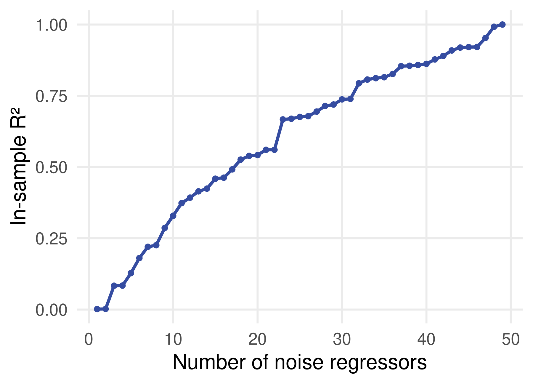
In-sample fit measures complexity as much as it measures signal.

With k noise regressors and n observations, the expected R-squared is about k/(n - 1), so the curve is close to a straight line. A perfect fit needs n - 1 regressors plus the intercept: n parameters for n observations.

The Lee (2008) election data

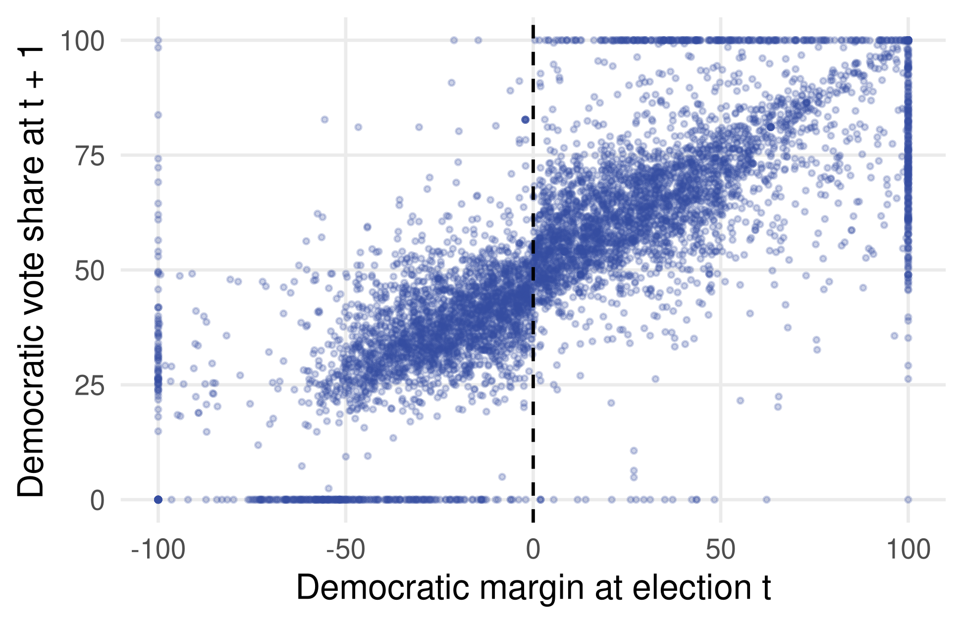
• X_i: the Democratic margin of victory in a U.S. House election, in percentage points, negative when the Democrat lost.
• Y_i: the Democratic vote share in the same district at the next election.
• 6,558 elections: 2,740 Democratic losses and 3,818 wins.
• Lee used the jump at a margin of zero to measure the incumbency advantage: a party that barely wins today keeps the seat tomorrow more often than one that barely loses. We return to this at the end of the next section.

ggplot(lee08, aes(margin, voteshare)) +
  geom_point(alpha = 0.25, size = 0.7, colour = smu_blue) +
  geom_vline(xintercept = 0, linetype = "dashed") +
  labs(x = "Democratic margin at election t",
       y = "Democratic vote share at t + 1")

[Sources] - Lee (2008), Randomized experiments from non-random selection in U.S. House elections, Journal of Econometrics 142, 675-697. Both variables are in percent. Many races are uncontested: 97 elections have a margin of -100 and 509 a margin of +100, which is why points pile up at the edges and why the bin cutpoints need de-duplication.

A simple predictor: the binned sample mean

Place the observations into d bins by the value of X_i: (t_0, t_1],\ (t_1, t_2],\ \dots,\ (t_{d-1}, t_d].

The prediction at x is the average outcome of the observations in the same bin as x: \hat f(x) = \frac{1}{n_j}\sum_{i:\ t_{j-1} < X_i \le t_j} Y_i \qquad \text{for } t_{j-1} < x \le t_j, \quad n_j = \#\{i: t_{j-1} < X_i \le t_j\}.

Three implementation choices for the election data:

• Zero is always a cutpoint, so no bin straddles the suspected jump.
• nbins bins on each side of zero, 2 \times nbins in total.
• Cutpoints are quantiles of X_i on each side, so every bin holds about the same number of elections.

This is the cell-mean idea from the regression lecture, with cells defined by bins of a continuous X.

The binned predictor in R

bin_cutpoints <- function(x_data, nbins) {
  x_neg <- sort(x_data[x_data < 0]); x_neg[length(x_neg)] <- 0   # make 0 a cutpoint
  x_pos <- sort(x_data[x_data > 0])
  unique(c(-Inf, x_neg[ceiling((1:nbins) * length(x_neg) / nbins)],   # quantile cutpoints,
                 x_pos[ceiling((1:nbins) * length(x_pos) / nbins)]))  # no empty bins
}
binned_predictor <- function(x_data, y_data, new_x, nbins) {
  cutpoints <- bin_cutpoints(x_data, nbins)
  means_by_bin <- tapply(y_data, cut(x_data, breaks = cutpoints), mean)
  means_by_bin[cut(new_x, breaks = cutpoints)]     # look up the bin of each new x
}
binned_predictor(lee08$margin, lee08$voteshare, new_x = c(-30, -1, 1, 30), nbins = 5)

## (-30.2,-19.5]     (-9.46,0]      (0,12.6]   (27.8,43.7] 
##      36.30102      43.33206      56.30646      67.91751

• cut() assigns each value to a bin (t_{j-1}, t_j], tapply() averages Y within bins, and indexing by the bins of new_x looks up the predictions.
• unique() drops duplicate cutpoints when many elections share a margin (the uncontested races at \pm 100), so the number of bins formed can be a little below 2 \times nbins.
• This is the function from the notes, split into a cutpoint step and a prediction step.

Ten bins: a step function with a jump at zero

xgrid <- seq(-100, 100, by = 0.1)
fit10 <- binned_predictor(lee08$margin, lee08$voteshare, new_x = xgrid, nbins = 5)
ggplot() +
  geom_point(data = lee08, aes(margin, voteshare), colour = "grey70", alpha = 0.4, size = 0.6) +
  geom_line(aes(xgrid, fit10), colour = smu_red, linewidth = 1) +
  labs(x = "Democratic margin at t", y = "Predicted vote share at t + 1")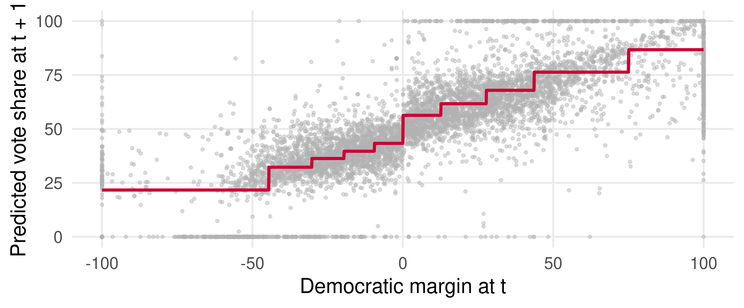

Each flat segment is a bin mean. Bins are narrow where elections are dense, near zero, and wide in the tails.

More bins, more complexity

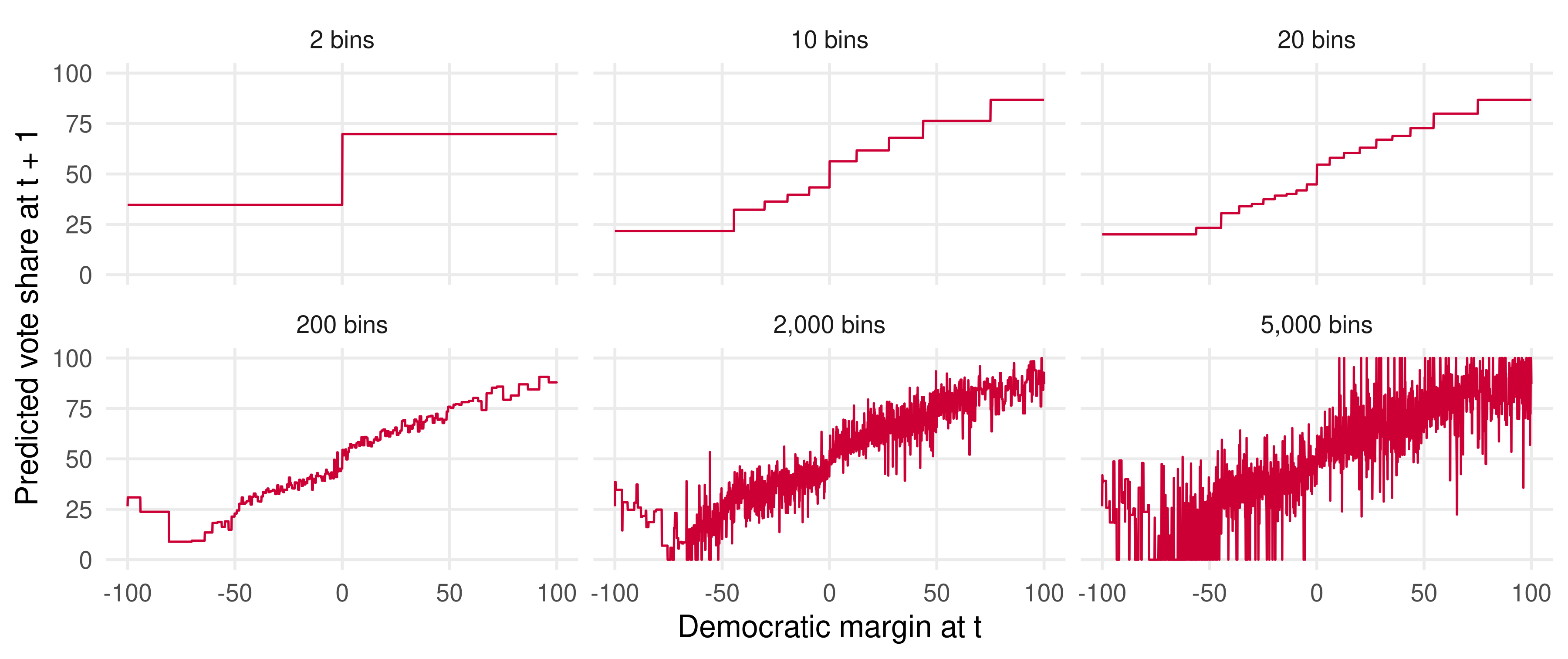
The same function with nbins = 1, 5, 10, 100, 1,000 and 2,500. At 5,000 bins almost every bin holds one election, and the “prediction” is the raw Y_i of whichever election is nearest.

Complexity is the number of parameters

In OLS, complexity is the number of coefficients. For the binned mean it is the number of bins, and the two are the same thing: the binned mean is a regression on bin indicators.

bin10 <- cut(lee08$margin, breaks = bin_cutpoints(lee08$margin, nbins = 5))  # factor, 10 levels
fit_lm <- lm(voteshare ~ bin10 - 1, data = lee08)      # one coefficient per bin, no intercept
max(abs(coef(fit_lm) - tapply(lee08$voteshare, bin10, mean)))

## [1] 1.563194e-13

• Each coefficient is the mean of Y in its bin. It is the regression on a factor from the linear regression lecture, with bins in place of brands.
• So 5,000 bins is a regression with about 4,500 coefficients on 6,558 observations, and the in-sample R^2 keeps rising with the number of bins, exactly as in the noise example.

Ties in the margin merge some cutpoints, so nbins = 2500 produces 4,491 bins rather than 5,000. The regression on dummies and the tapply means agree to machine precision.

R2

tibble(nbins = c(1, 5, 10, 100, 1000, 2500)) %>%
  mutate(bins = 2 * nbins, in_sample_r2 = map_dbl(nbins, r2_in)) %>%
  knitr::kable(digits = 3)

nbins	bins	in_sample_r2
1	2	0.517
5	10	0.673
10	20	0.678
100	200	0.692
1000	2000	0.761
2500	5000	0.878

• The in-sample R^2 rises with every added bin and would reach 1 with one election per bin.
• The 200-bin picture already looked noisy, but “looks noisy” is a judgment, not a criterion.
• We need a number that measures how a fitted model does on data it was not fitted to.

r2_in() computes 1 - deviance / null deviance on the full sample; it was defined for the opening slide. The last row has 4,491 bins formed, so R-squared is 0.88 rather than 1.

Checkpoint: overfitting

1. Why can adding a regressor never lower the in-sample R^2 of an OLS regression?
2. A colleague fits a regression with 300 dummies to 400 observations and reports R^2 = 0.9. What do you want to know before being impressed?
3. In the binned mean, what plays the role of “number of covariates”? What is the prediction at a new x when every bin holds one observation?

Answers: the smaller model is nested in the larger one, so the minimized sum of squares cannot increase; how the model does out of sample, since 300 pure-noise dummies alone would give an R-squared of roughly 300/399 = 0.75; the number of bins, and the prediction is the outcome of the single election in that bin, noise included.

Out-of-sample fit and cross-validation

---

Measure prediction error on data the model never saw

Out-of-sample deviance

The in-sample deviance for least squares, fitted on i = 1, \dots, n: \text{dev}_{IS}(\hat\beta) = \sum_{i=1}^n (Y_i - X_i'\hat\beta)^2.

Suppose m new observations arrive, labelled n+1, \dots, n+m. The out-of-sample deviance is \text{dev}_{OOS}(\hat\beta) = \sum_{i=n+1}^{n+m} (Y_i - X_i'\hat\beta)^2.

• \hat\beta is computed from the first n observations only. Refitting on all n + m would turn this into an in-sample deviance for a bigger sample.
• For the binned mean, replace X_i'\hat\beta by \hat f(X_i), with bins and bin means computed from the first n observations.

Out-of-sample R^2

R^2_{OOS} = 1 - \frac{\text{dev}_{OOS}(\hat\beta)}{\text{dev}_{OOS}(\hat\beta_{\text{null}})}, \qquad \text{dev}_{OOS}(\hat\beta_{\text{null}}) = \sum_{i=n+1}^{n+m} (Y_i - \bar Y)^2,

where \bar Y is the mean of the estimation sample, the prediction of the no-covariate model.

• This is literally how the predictions fare on new data, so it is the right measure of predictive performance.
• R^2_{OOS} can be negative: a model that chases noise can predict worse than \bar Y.
• How far apart can R^2 and R^2_{OOS} be? Hold out part of the sample and find out.

A single split of the election data

set.seed(0)
n <- nrow(lee08)
est <- sample.int(n, size = round(2 * n / 3))    # 4,372 elections to fit, 2,186 to test
x_est <- lee08$margin[est];   y_est <- lee08$voteshare[est]
x_test <- lee08$margin[-est]; y_test <- lee08$voteshare[-est]
r2_split <- function(nbins) {
  fit_in  <- binned_predictor(x_est, y_est, new_x = x_est,  nbins)
  fit_out <- binned_predictor(x_est, y_est, new_x = x_test, nbins)
  tibble(bins = 2 * nbins,
         in_sample     = 1 - sum((y_est - fit_in)^2)   / sum((y_est - mean(y_est))^2),
         out_of_sample = 1 - sum((y_test - fit_out)^2) / sum((y_test - mean(y_est))^2))
}
r2_split(nbins = 5)

## # A tibble: 1 × 3
##    bins in_sample out_of_sample
##   <dbl>     <dbl>         <dbl>
## 1    10     0.662         0.693

• The estimation sample plays the role of the first n observations and the test sample of the m new ones.
• Both R^2 use \bar Y from the estimation sample, so the out-of-sample version is exactly R^2_{OOS}.

In-sample and out-of-sample R^2 by number of bins

split_tab <- map_dfr(c(5, 10, 100, 1000, 2500), r2_split)
knitr::kable(split_tab, digits = 3)

bins	in_sample	out_of_sample
10	0.662	0.693
20	0.668	0.697
200	0.688	0.693
2000	0.796	0.587
5000	0.935	0.448

• In-sample R^2 climbs with every bin, to above 0.93 at 5,000 bins.
• Out-of-sample R^2 peaks near 0.70 at 20 to 200 bins and falls to 0.45 at 5,000 bins: the model with the best in-sample fit predicts worst.

The two curves part ways

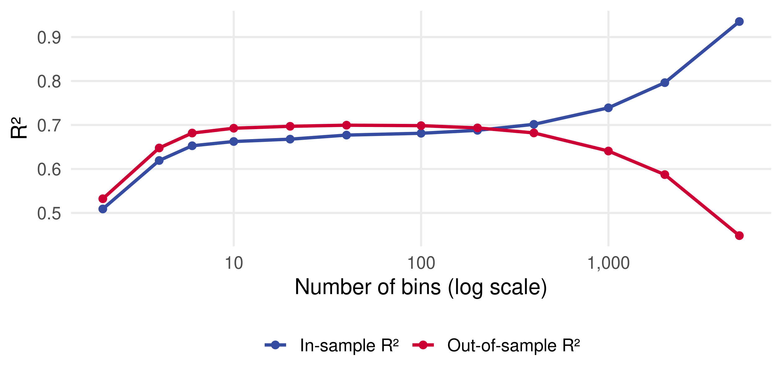
• In-sample R^2 rises with every bin, from 0.51 at 2 bins to above 0.93 at 5,000.
• Out-of-sample R^2 rises until about 20 bins, stays near 0.70 up to 200 bins, then collapses as the bins empty out. The gap between the curves is the overfitting.

For few bins the two measures agree up to sampling noise; in this split the out-of-sample value is even slightly higher for 10 to 100 bins, which is not a contradiction. The split also fits on only two thirds of the data, so its out-of-sample R-squared is slightly pessimistic for the full-sample model.

One split is a noisy estimate

oos_r2 <- function(seed, nbins = 100) {
  set.seed(seed)
  est <- sample.int(n, size = round(2 * n / 3))
  fit <- binned_predictor(lee08$margin[est], lee08$voteshare[est], lee08$margin[-est], nbins)
  1 - sum((lee08$voteshare[-est] - fit)^2) /
      sum((lee08$voteshare[-est] - mean(lee08$voteshare[est]))^2)
}
round(sapply(1:10, oos_r2), 3)

##  [1] 0.677 0.690 0.673 0.651 0.716 0.658 0.679 0.686 0.672 0.660

• The same 200-bin model scores anywhere between 0.65 and 0.72, depending on which third of the sample is held out.
• The ranking of two models can flip from one split to the next, so a single split is a shaky basis for model selection.
• The fix: repeat the split several times and average. That is K-fold cross-validation.

K-fold cross-validation

Step 1. Split the data at random into K folds of (almost) equal size.

Step 2. For each k = 1, \dots, K, fit the model on all folds except the kth, giving a predictor \hat f_{-k}, and score it on fold k: \text{dev}_{OOS,k} = \sum_{i \in \text{fold } k} \big(Y_i - \hat f_{-k}(X_i)\big)^2.

Step 3. Average the K out-of-sample deviances: \text{dev}_{CV} = \frac{1}{K}\sum_{k=1}^K \text{dev}_{OOS,k}.

Every observation is predicted exactly once, by a model that did not see it. We report the result per observation, as a mean squared prediction error.

Five folds, five test sets

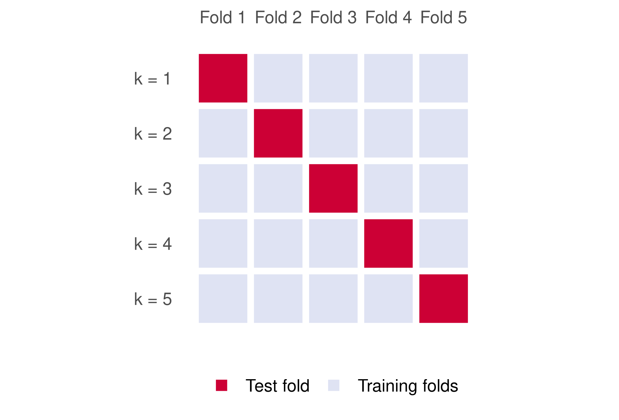
• Each row is one round: the red block is the test fold, the others are the training folds.
• Every observation is in the test fold exactly once and in the training folds K - 1 times.
• The K out-of-sample errors are averaged; their spread gives a standard error for the average.
• K = 5 and K = 10 are the usual choices. K = n is leave-one-out CV (appendix).

[Sources] - Hastie, Tibshirani and Friedman (2009), The Elements of Statistical Learning, section 7.10.1, whose diagram this slide reproduces; the notes embed the original as images/cv_illustration_hastie_et_al_2008.png.

Assign the folds in R

set.seed(0)
K <- 10
foldid <- rep(1:K, each = ceiling(n / K))[sample(1:n)]
table(foldid)

## foldid
##   1   2   3   4   5   6   7   8   9  10 
## 656 656 656 656 656 656 656 656 656 654

• rep(1:K, each = ceiling(n / K)) writes the labels 1, 1, \dots, 1, 2, 2, \dots, K: ten blocks of 656, slightly more than n = 6{,}558 labels.
• sample(1:n) is a random permutation of 1, \dots, n. Indexing by it shuffles the labels, keeps n of them and drops the rest.
• Each fold has 656 or 654 elections. Run the two pieces separately to see what each one does.

The cross-validation loop

nbins_vec <- 1:250                   # 2 to 500 bins: more was clearly worse in the single split
cv_mat <- matrix(NA, nrow = K, ncol = length(nbins_vec))   # row k: fold k held out
for (i in seq_along(nbins_vec)) {
  for (k in 1:K) {
    train <- which(foldid != k)
    fit_k <- binned_predictor(lee08$margin[train], lee08$voteshare[train],
                              new_x = lee08$margin[-train], nbins = nbins_vec[i])
    cv_mat[k, i] <- mean((lee08$voteshare[-train] - fit_k)^2)
  }
}
cv_error <- colMeans(cv_mat)                 # K-fold CV estimate for each candidate
cv_se <- apply(cv_mat, 2, sd) / sqrt(K)      # standard error of that average across folds
nbins_cv <- nbins_vec[which.min(cv_error)]
c(bins_chosen = 2 * nbins_cv, cv_error = min(cv_error), se = cv_se[nbins_cv])

## bins_chosen    cv_error          se 
##   46.000000  184.421240    4.345252

• 250 candidate models times 10 folds is 2,500 fits; the loop runs in a few seconds.
• cv_mat[k, i] is the mean squared prediction error on fold k for candidate i. The column mean is \text{dev}_{CV} per observation.

Cross-validation picks 46 bins

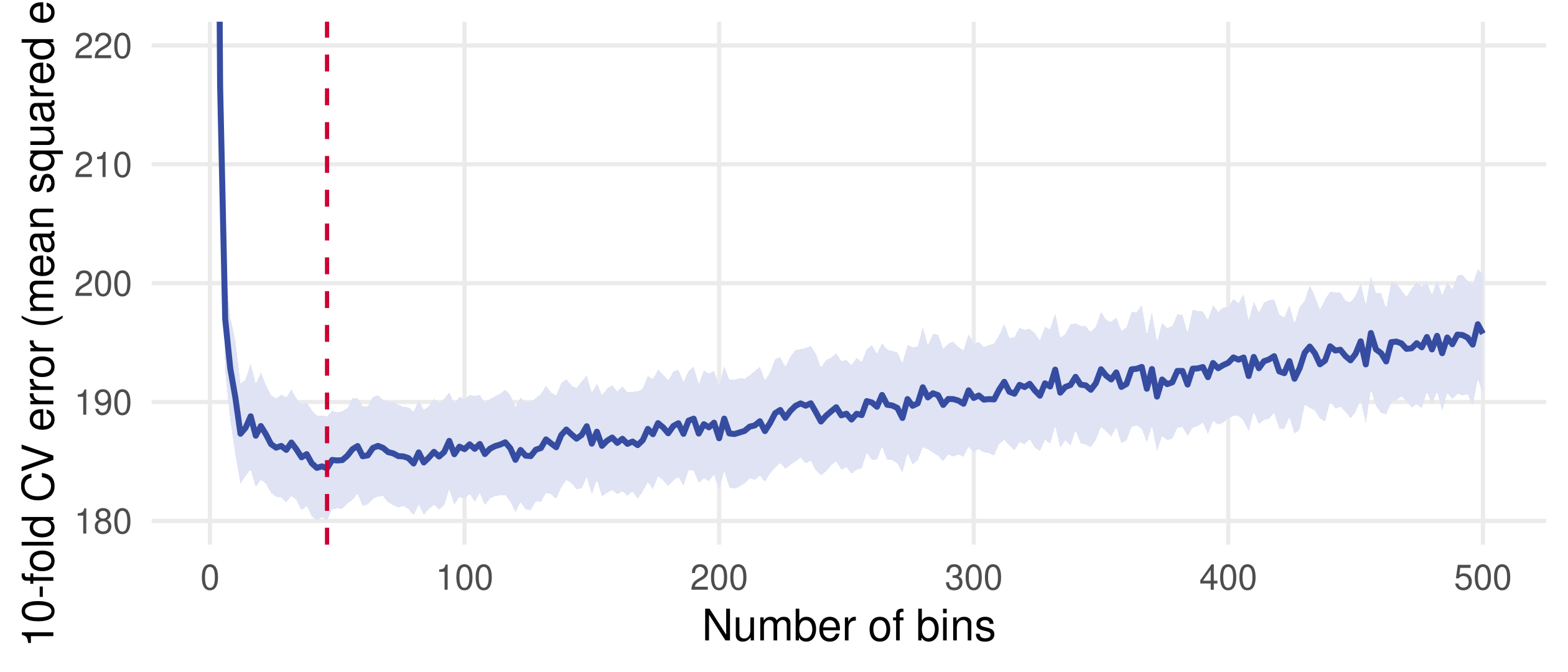
• The minimum, 184.4, is at 46 bins. The band is one standard error across the ten folds, about 4.3.
• The valley is flat: every choice from 26 to 136 bins is within 1% of the minimum. At 2 bins the error is 281, off the chart; beyond 150 bins it climbs steadily.
• Other fold assignments put the minimum between 42 and 46 bins (appendix). The region matters more than the point.

The predictor cross-validation chose

fit_cv <- binned_predictor(lee08$margin, lee08$voteshare, new_x = xgrid, nbins = nbins_cv)

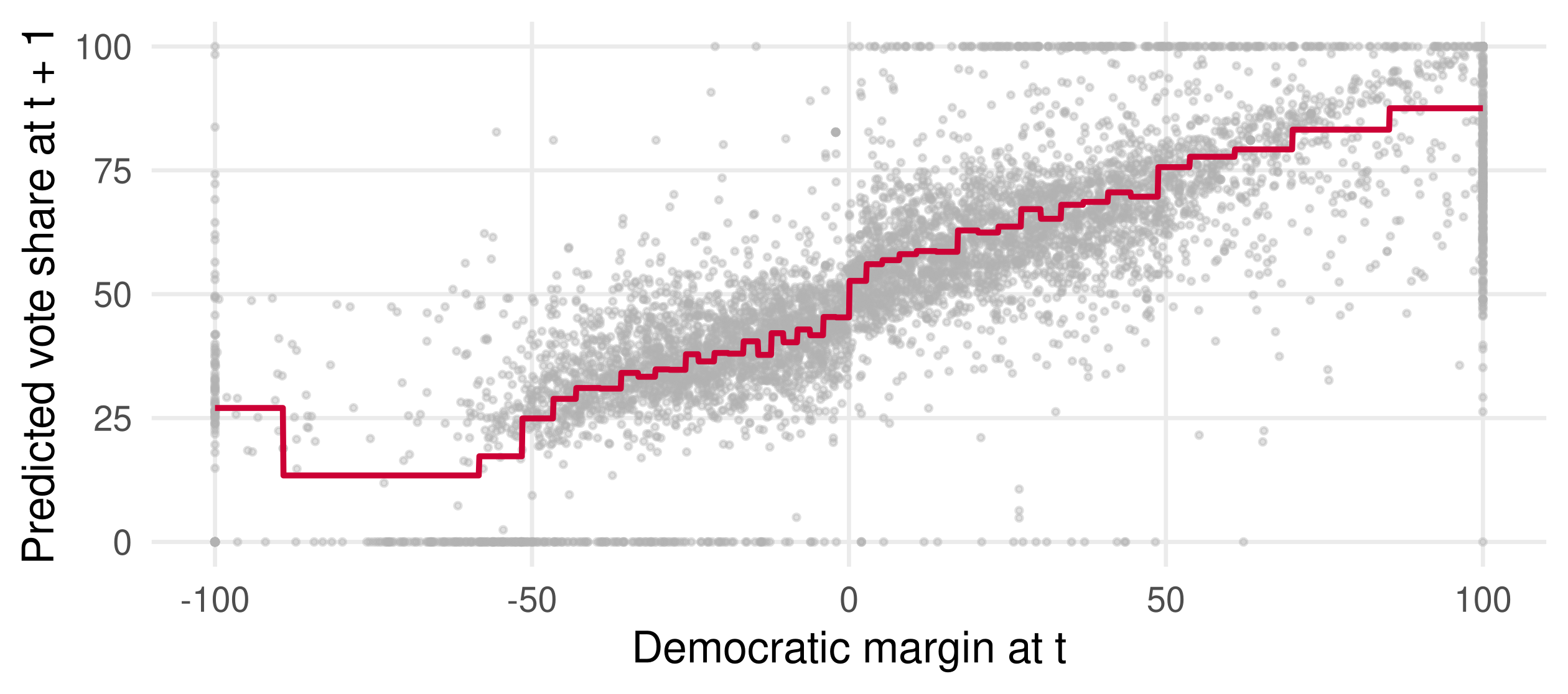
Refitted on the full sample with the chosen 23 bins on each side of zero, using the same plotting code as the ten-bin slide. The staircase is fine where elections are dense, and the jump at zero survives.

Cross-validation as a model-selection recipe

1. Index the candidate models by a tuning parameter: the number of bins here, the number of regressors, the penalty \lambda of a lasso next lecture, the depth of a tree after that.
2. Compute the CV error for every value of the tuning parameter.
3. Pick the value with the smallest CV error, or the simplest model within one standard error of the minimum.

within_1se <- cv_error <= min(cv_error) + cv_se[nbins_cv]
c(min_rule = 2 * nbins_cv, one_se_rule = 2 * nbins_vec[which(within_1se)[1]])

##    min_rule one_se_rule 
##          46          12

• The one-standard-error rule picks 12 bins: a much simpler model whose CV error of 187.3 is statistically indistinguishable from the best.
• cv.glmnet() reports both choices next lecture, as lambda.min and lambda.1se.

Choosing K

K	Training size	Properties
2	n/2	Cheap; pessimistic, since each model sees half the data
5 or 10	0.8\,n or 0.9\,n	The standard choices
n (leave-one-out)	n - 1	Closest to the full-sample model; n fits, and the n errors are highly correlated

• K-fold CV estimates the error of a model fitted on n(K-1)/K observations, slightly fewer than the final model will use, so it is mildly pessimistic.
• For the election data, 5-fold and 10-fold both choose 46 bins and leave-one-out chooses 44 (appendix).
• Repeating CV with different random fold assignments and averaging reduces the noise further.

Checkpoint: cross-validation

1. In 10-fold CV with n = 6{,}558 elections, how many times is each election predicted out of sample, and how many models are fitted per candidate?
2. Suppose the folds were formed by sorting on the margin: fold 1 holds the most negative margins, fold 10 the most positive. Why would the CV error mislead?
3. Two candidates have CV errors of 184.4 and 186.0 with standard errors around 4.3. Is the first clearly better?

Answers: once, and ten; the training set would not cover the test fold’s range of X, so the predictions come from the nearest bin (or are missing) and the exercise no longer mimics predicting new elections drawn like the old ones; no, the difference is well inside one standard error, which is the logic behind the one-standard-error rule.

The bias-variance trade-off

---

Why cross-validation works, and why complexity cuts both ways

The population mean squared error

Posit Y = f(X) + \varepsilon with \mathbf{E}[\varepsilon \mid X] = 0. Linear regression is the case f(x) = x'\beta; the binned mean, trees and neural networks estimate more flexible f.

Let \hat f be an estimator computed from the sample (X_1, Y_1), \dots, (X_n, Y_n), and (X_{n+1}, Y_{n+1}) a new draw from the same population. The population mean squared error is

\text{MSE} = \mathbf{E}\big[(Y_{n+1} - \hat f(X_{n+1}))^2\big].

The expectation averages over two sources of randomness:

• the sample, which makes \hat f random: estimation error, how far \hat f is from f;
• the new observation: irreducible error, since even f(X_{n+1}) misses Y_{n+1} by \varepsilon_{n+1}.

Out-of-sample error estimates the population MSE

For m new observations, \mathbf{E}\left[\frac{1}{m}\,\text{dev}_{OOS}\right] = \frac{1}{m}\sum_{i=n+1}^{n+m} \mathbf{E}\big[(Y_i - \hat f(X_i))^2\big] = \text{MSE}.

• The out-of-sample deviance per observation is an unbiased estimate of the population MSE: it is what the model’s error will be “on average” over samples and new draws.
• K-fold CV produces K such estimates, one per fold, and averages them. Averages approximate expectations by the law of large numbers, so the CV error approximates the MSE. This is the mathematical reason CV works.
• The standard-error band on the CV plot is the sampling noise in that approximation.
• Strictly, the \hat f_{-k} use n(K-1)/K observations, so CV approximates the MSE of a model fitted on slightly less data.

Step 1: irreducible error plus estimation error

\begin{aligned} \mathbf{E}\big[(Y_{n+1} - \hat f(X_{n+1}))^2\big] &= \mathbf{E}\big[(\varepsilon_{n+1} + f(X_{n+1}) - \hat f(X_{n+1}))^2\big] \\ &= \underbrace{\mathbf{E}[\varepsilon_{n+1}^2]}_{\text{irreducible error}} + \underbrace{\mathbf{E}\big[(\hat f(X_{n+1}) - f(X_{n+1}))^2\big]}_{\text{estimation error}} + 2\,\mathbf{E}\big[\varepsilon_{n+1}\big(f(X_{n+1}) - \hat f(X_{n+1})\big)\big]. \end{aligned}

The cross term is zero: \hat f depends on the sample only, and \varepsilon_{n+1} is a fresh mean-zero draw, so that \mathbf{E}[\varepsilon_{n+1} \mid \text{sample}, X_{n+1}] = 0.

• The irreducible error \sigma^2 = \mathbf{E}[\varepsilon^2] is the same for every estimator. No model, however complex, can predict the noise.
• Everything we can influence sits in the estimation error.

Step 2: estimation error is variance plus squared bias

Fix x and add and subtract \mathbf{E}[\hat f(x)], the average of \hat f(x) over samples:

\begin{aligned} \mathbf{E}\big[(\hat f(x) - f(x))^2\big] &= \mathbf{E}\Big[\big(\hat f(x) - \mathbf{E}[\hat f(x)] + \mathbf{E}[\hat f(x)] - f(x)\big)^2\Big] \\ &= \underbrace{\mathbf{E}\Big[\big(\hat f(x) - \mathbf{E}[\hat f(x)]\big)^2\Big]}_{V(x):\ \text{variance}} + \underbrace{\big(\mathbf{E}[\hat f(x)] - f(x)\big)^2}_{B(x)^2:\ \text{squared bias}}, \end{aligned}

since the cross term is 2\,\big(\mathbf{E}[\hat f(x)] - f(x)\big)\,\mathbf{E}\big[\hat f(x) - \mathbf{E}[\hat f(x)]\big] = 0.

• Bias B(x): how far the estimator is from the truth on average across samples. Systematic error.
• Variance V(x): how much the estimator moves from sample to sample. Random error.

Put together: three components

Averaging over the distribution of the new X_{n+1}, \text{MSE} = \underbrace{\sigma^2}_{\text{irreducible}} + \underbrace{\mathbf{E}[V(X_{n+1})]}_{\text{variance}} + \underbrace{\mathbf{E}[B(X_{n+1})^2]}_{\text{squared bias}}.

Component	Where it comes from	Can we reduce it?
Irreducible error	Noise in Y given X	No. Only better predictors X help.
Variance	The particular sample we drew	Yes: a simpler model, or more data
Squared bias	The model’s inability to represent f	Yes: a more flexible model

No need to memorize the algebra. The point is that the two reducible components move in opposite directions when we change the complexity of the model.

The trade-off

• A more complex model (more regressors, more bins, a deeper tree) can approximate f better: lower bias.
• A more complex model has more parameters to estimate from the same data: higher variance.
• The MSE is minimized somewhere in between, and cross-validation is how we locate that point from data.

Next lecture adds a knob that runs the other way, a penalty \lambda on the size of the coefficients:

\text{penalization } \lambda \uparrow \;\Longrightarrow\; \text{complexity} \downarrow \;\Longrightarrow\; \text{bias} \uparrow,\ \text{variance} \downarrow.

In the extreme \lambda \to \infty, \hat\beta \to 0 and we predict Y_{n+1} = 0 without looking at the data: zero variance, large bias (unless f = 0).

A simulation where we know the truth

set.seed(0)
n_sim <- 500
x_sim <- runif(n_sim)                       # all positive: the zero cutpoint plays no role
y_sim <- 1 + x_sim + 0.2 * rnorm(n_sim)     # f(x) = 1 + x, irreducible error 0.2^2 = 0.04

• The true conditional mean is the line f(x) = 1 + x and \sigma^2 = 0.04. Because we can draw as many samples as we like, bias and variance can be computed rather than imagined.
• With every X_i > 0, nbins is simply the number of bins, and the binned mean approximates a line with a staircase.

One sample, five bin counts

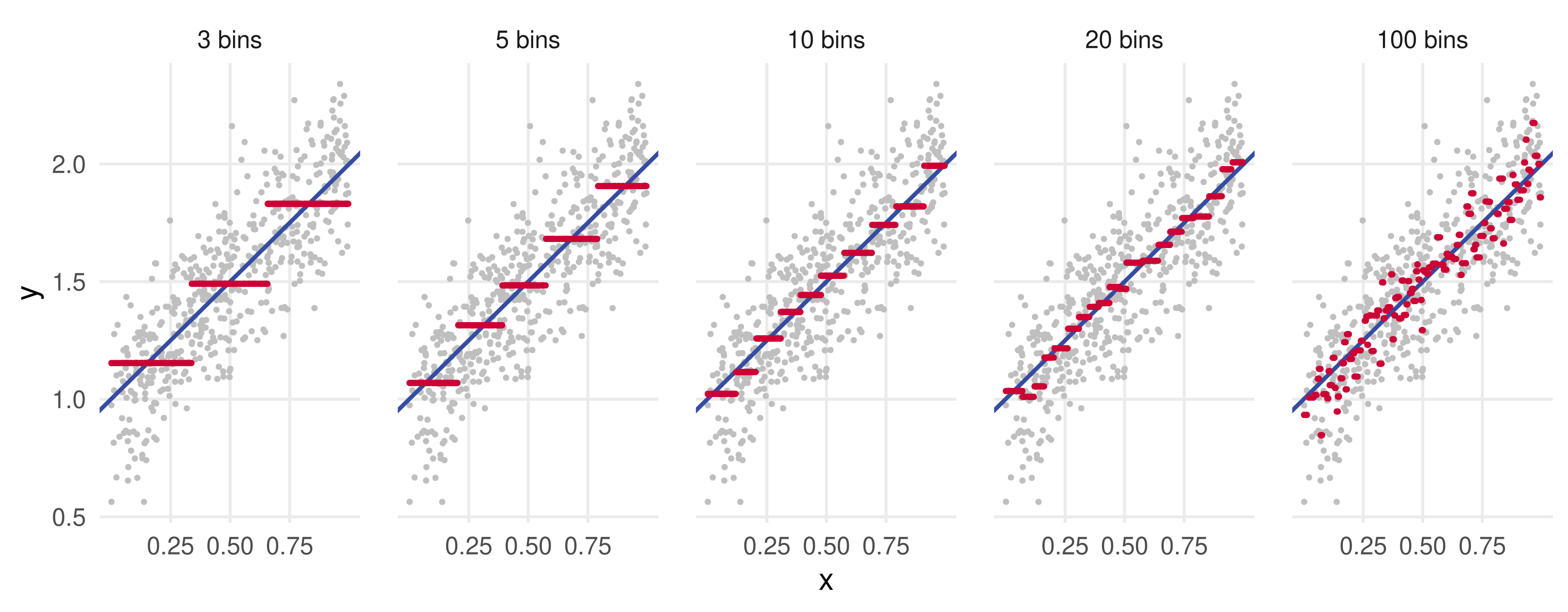
• Few bins: the staircase cannot follow the line. At the left end of every bin the estimate is too high, at the right end too low. That is bias, and it is the same in every sample.
• Many bins: the steps are short enough to track the line, but each is the average of a handful of noisy points and jumps around it. That is variance, different in every sample.

Repeat the experiment 300 times

R <- 300
grid <- seq(0.025, 0.975, length.out = 191)          # where the fits are evaluated
bins_sim <- c(1, 2, 3, 5, 10, 20, 50, 100)
fits <- array(NA, dim = c(R, length(grid), length(bins_sim)))
for (r in 1:R) {
  x <- runif(n_sim); y <- 1 + x + 0.2 * rnorm(n_sim)   # a fresh sample each time
  for (j in seq_along(bins_sim))
    fits[r, , j] <- binned_predictor(x, y, new_x = grid, nbins = bins_sim[j])
}
bias_var <- map_dfr(seq_along(bins_sim), function(j) {
  avg_fit <- colMeans(fits[, , j])                     # E[f_hat(x)] at each grid point
  tibble(bins = bins_sim[j],
         bias2 = mean((avg_fit - (1 + grid))^2),       # B(x)^2 averaged over the grid
         variance = mean(apply(fits[, , j], 2, var)))  # V(x) averaged over the grid
}) %>% mutate(mse = bias2 + variance + 0.2^2)

• fits[r, , j] holds sample r’s fit with bins_sim[j] bins along the grid. The mean over r approximates \mathbf{E}[\hat f(x)] and the variance over r approximates V(x).
• The grid stays inside (0.025, 0.975) so that every grid point falls within the range of each sample.

Average fit against the truth: bias. Spread: variance.

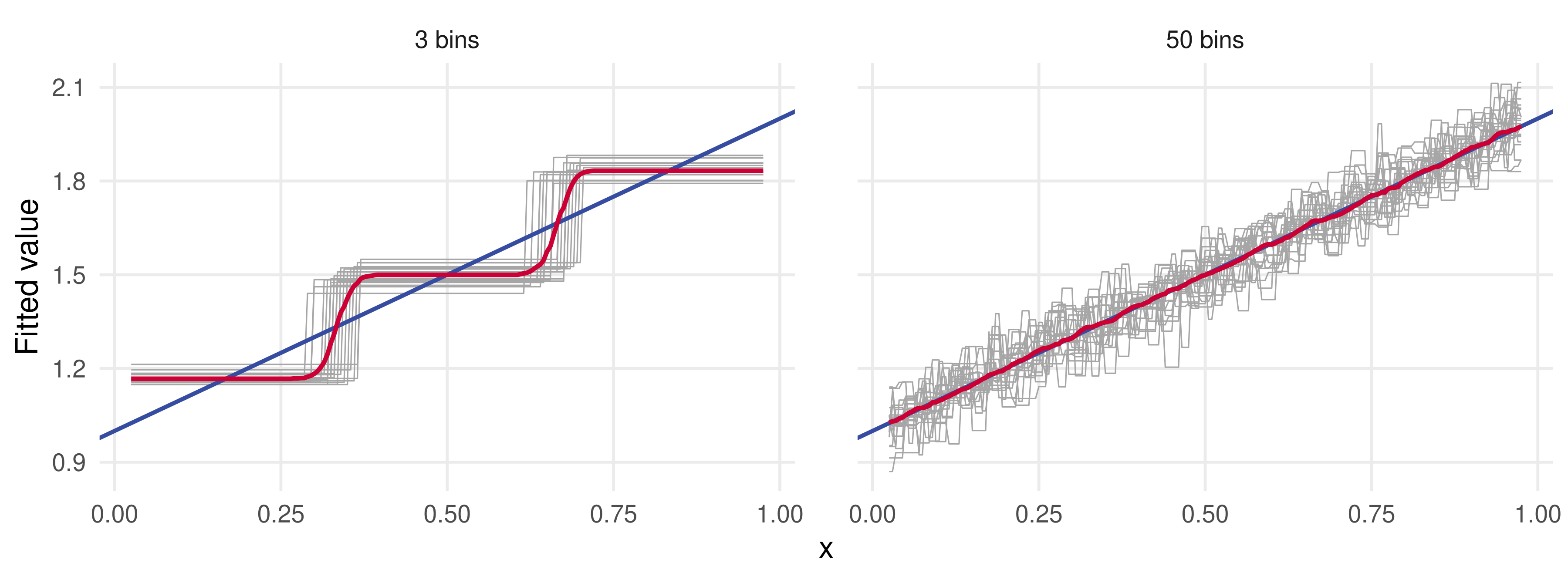
Grey: fits from 20 different samples. Red: the average fit over all 300. Blue: the truth. With 3 bins the average is a staircase far from the line and the grey fits lie on top of each other: bias without variance. With 50 bins the average sits on the line but the individual fits scatter: variance without bias.

Bias falls, variance rises, and their sum is U-shaped

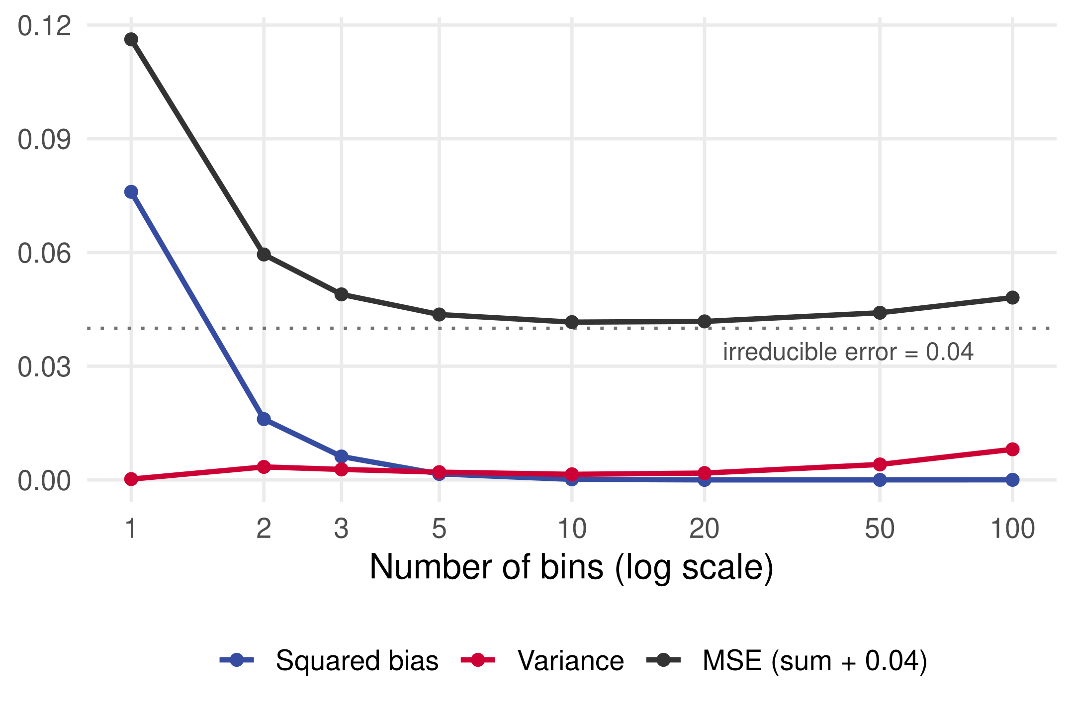
bins	bias2	variance	mse
1	0.0760	0.0002	0.1162
2	0.0160	0.0034	0.0595
3	0.0062	0.0028	0.0489
5	0.0016	0.0021	0.0436
10	0.0001	0.0015	0.0416
20	0.0000	0.0018	0.0418
50	0.0000	0.0041	0.0441
100	0.0000	0.0081	0.0481

The MSE is smallest at 10 bins, 0.0416, just above the floor of 0.04 set by the noise. Fewer bins pay in bias, more bins pay in variance.

If you know the truth is linear, say so

ols_fits <- matrix(NA, nrow = R, ncol = length(grid))
for (r in 1:R) {
  x <- runif(n_sim); y <- 1 + x + 0.2 * rnorm(n_sim)
  b <- coef(lm(y ~ x)); ols_fits[r, ] <- b[1] + b[2] * grid
}
c(bias2 = mean((colMeans(ols_fits) - (1 + grid))^2), variance = mean(apply(ols_fits, 2, var)))

##        bias2     variance 
## 4.848163e-07 1.529540e-04

• OLS on an intercept and x has no bias (the model is right) and a variance ten times smaller than the best binned mean: MSE 0.0402 against 0.0416. That is the value of a correct parametric restriction.
• But if f were curved, the line would be biased at every x, and no sample size would fix it. A wrong restriction buys variance reduction with permanent bias.
• In practice we rarely know f. Flexible methods plus cross-validation trade a little variance for insurance against bias, and each step up in complexity usually buys a little less bias reduction than the last.

Checkpoint: bias and variance

1. You double the sample size and keep 10 bins. Which component of the MSE falls, and which stay the same?
2. A predictor returns \bar Y regardless of x. Describe its bias and its variance.
3. Why does the CV curve on the election data have the same U shape as the simulation’s MSE curve?

Answers: the variance falls because each bin averages twice as many observations, while the bias (the same staircase) and the irreducible error are unchanged; it has the smallest possible variance for a data-based predictor, and a bias equal to f(x) minus the overall mean, large wherever f varies; the CV error estimates the population MSE, which is irreducible error plus variance plus squared bias, and the number of bins trades the last two exactly as in the simulation.

Information criteria

---

A formula in place of the cross-validation loop

Why the in-sample deviance is too optimistic

\begin{aligned} \text{dev}_{IS} &= \sum_{i=1}^n (Y_i - \hat f(X_i))^2 = \sum_{i=1}^n \big(Y_i - f(X_i) + f(X_i) - \hat f(X_i)\big)^2 \\ &= \underbrace{\sum_{i=1}^n (Y_i - f(X_i))^2}_{\text{noise}} + \underbrace{\sum_{i=1}^n (\hat f(X_i) - f(X_i))^2}_{\text{estimation error}} - 2 \underbrace{\sum_{i=1}^n (Y_i - f(X_i))\big(\hat f(X_i) - f(X_i)\big)}_{\text{the overfitting term}}. \end{aligned}

• The last term is positive on average whenever \hat f(X_i) moves with \varepsilon_i = Y_i - f(X_i): the fit “cheats” by using Y_i to predict Y_i. More complexity means more cheating and a smaller \text{dev}_{IS}.
• Cross-validation removes the term by predicting each Y_i with a model that never saw it.
• An information criterion keeps the in-sample fit and adds an estimate of the term back.

Degrees of freedom

For least squares, define the degrees of freedom of an estimator as df = \frac{1}{\sigma^2}\,\mathbf{E}\left[\sum_{i=1}^n (Y_i - f(X_i))\big(\hat f(X_i) - f(X_i)\big)\right], \qquad \sigma^2 = \mathbf{E}[\varepsilon_i^2], so the overfitting term is 2\,\sigma^2 df on average.

Estimator	df
OLS, logit, other maximum likelihood estimators	Number of parameters
Binned mean	Number of bins
Lasso	Number of nonzero coefficients (a deep result; next lecture)
Ridge	A formula in \lambda and the design matrix

• Under normal errors a general formula exists (Stein’s lemma; appendix).
• summary() of an lm reports residual degrees of freedom, n - df, not df.

Likelihood models use the same name for the analogous quantity, which is what AIC uses. For OLS the residual degrees of freedom are n minus the number of coefficients, so summary() gives n - df, not df.

Mallows’ C_p, AIC and AICc

Adding the estimated overfitting term to the deviance gives Mallows’ C_p: C_p = \frac{1}{\hat\sigma^2}\sum_{i=1}^n (Y_i - \hat f(X_i))^2 + 2\,df, with \hat\sigma^2 taken from a low-bias model (many bins, or all available regressors).

For likelihood models, Akaike’s information criterion has the same shape, \text{AIC}(\hat f) = \text{dev}_{IS}(\hat f) + 2\,df, and reduces to C_p for a Gaussian likelihood with \sigma^2 treated as known. The corrected AIC inflates the penalty when df is not small relative to n, which also accounts for estimating \sigma^2: \text{AICc}(\hat f) = \text{dev}_{IS}(\hat f) + 2\,df\,\frac{n}{n - df - 1}.

Smaller is better. Packages differ in constants and normalizations, so compare AIC values only within one routine.

C_p for the binned predictor

dev_df <- function(nbins) {
  fit <- binned_predictor(lee08$margin, lee08$voteshare, new_x = lee08$margin, nbins)
  tibble(bins = 2 * nbins, dev = sum((lee08$voteshare - fit)^2),
         df = length(bin_cutpoints(lee08$margin, nbins)) - 1)   # bins actually formed
}
ic <- map_dfr(nbins_vec, dev_df)
sigma2_hat <- with(ic[250, ], dev / (n - df))          # from the 500-bin, low-bias model
ic <- ic %>% mutate(cp = dev / sigma2_hat + 2 * df,
                    cp_as_mse = cp * sigma2_hat / n)   # same ranking, on the CV error's scale
c(sigma2_hat = sigma2_hat, bins_cp = ic$bins[which.min(ic$cp)], bins_cv = 2 * nbins_cv)

## sigma2_hat    bins_cp    bins_cv 
##   184.5481    44.0000    46.0000

• df counts the bins actually formed, since ties in the margin merge some cutpoints.
• Multiplying C_p by \hat\sigma^2/n gives \text{dev}_{IS}/n + 2\,df\,\hat\sigma^2/n: the in-sample MSE plus the estimated overfitting term per observation, directly comparable with the CV error.
• C_p chooses 44 bins where CV chose 46. AICc also picks 44.

C_p tracks the CV curve

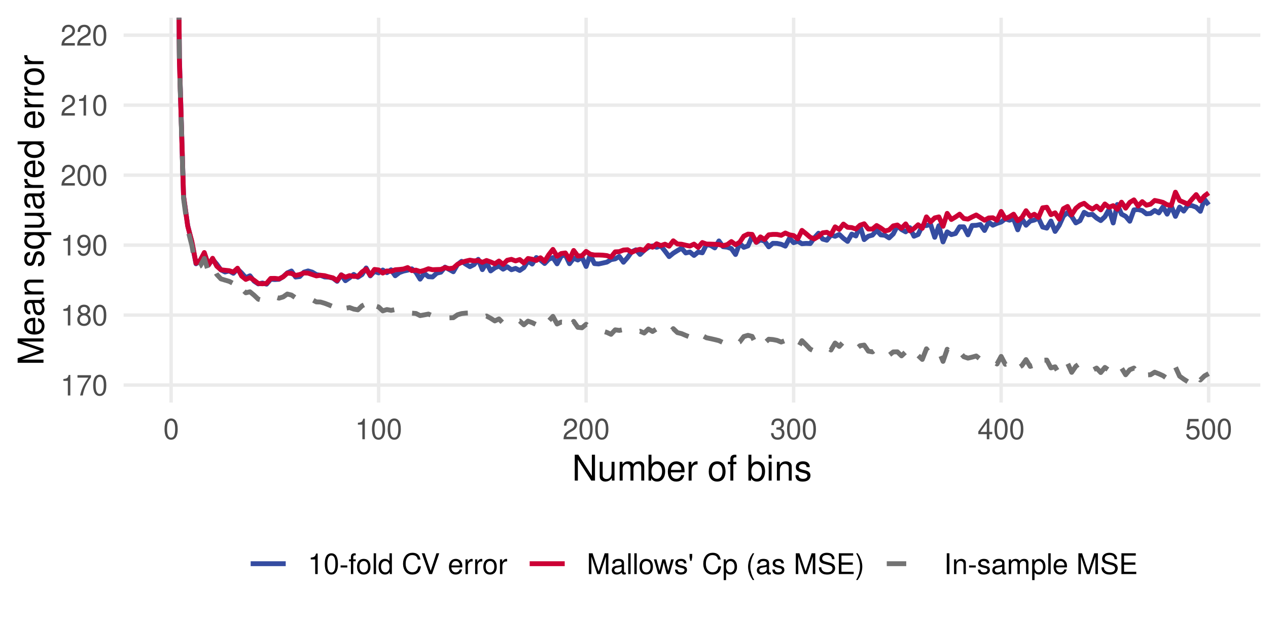
• The in-sample MSE falls forever. Adding 2\,df\,\hat\sigma^2/n bends it into a U that lies almost on top of the CV curve: the correlation across the 250 candidates is 0.99.
• No refitting was needed: one pass over the data instead of ten.

AIC versus cross-validation

	Cross-validation	AIC and C_p
Estimates	Population MSE of a model fitted on n(K-1)/K observations	Expected error of predicting a new Y at the sample’s X_i (appendix)
Needs	Only the ability to refit the model	A df formula; for the theory, homoskedastic (and often normal) errors
Cost	K fits per candidate	One fit per candidate
Scope	Any predictor, any loss function	Likelihood-based models with a known df

Both estimate out-of-sample performance from a single sample, and both are used the same way: compute the criterion along the candidates and take the minimum. AIC is a computational shortcut to CV, with a slightly different target and stronger assumptions.

Prediction is judged out of sample

In-sample fit rewards complexity. R^2 rises with every added parameter, even pure noise, and a model that tracks \varepsilon_i predicts nothing.

Out-of-sample error is the criterion. Hold data out, predict it, and score the predictions. K-fold cross-validation does this once for every observation and averages the result.

Cross-validation estimates the population MSE. The MSE is irreducible error plus variance plus squared bias, and complexity trades the last two against each other.

Information criteria are the shortcut. AIC and C_p add 2\,df to the in-sample deviance to undo its optimism, and they track the CV curve closely at a fraction of the cost.

Choose the tuning parameter for the target. CV optimizes average prediction. A local parameter such as the incumbency jump needs its own criterion.

Reading and data sources

• James, Witten, Hastie and Tibshirani, An Introduction to Statistical Learning, chapter 2 (bias and variance) and chapter 5 (cross-validation).
• Hastie, Tibshirani and Friedman, The Elements of Statistical Learning, chapter 7: model assessment and selection, including C_p, AIC, effective degrees of freedom and cross-validation.
• Lee (2008), Randomized experiments from non-random selection in U.S. House elections, Journal of Econometrics 142, 675-697: the election data and the incumbency design.
• RDHonest (Kolesár): the lee08 data set and the regression discontinuity estimator used for comparison, from Armstrong and Kolesár (2020), Quantitative Economics 11, 1-39.
• Wasserman’s note on Stein’s lemma: where the degrees-of-freedom formula comes from.

Additional derivations and code

---

Optional material for reference and practice

The CV choice under other fold assignments

cv_choice <- function(seed) {
  set.seed(seed)
  foldid <- rep(1:K, each = ceiling(n / K))[sample(1:n)]
  err <- sapply(nbins_vec, function(nb) mean(sapply(1:K, function(k) {
    train <- which(foldid != k)
    fit_k <- binned_predictor(lee08$margin[train], lee08$voteshare[train],
                              new_x = lee08$margin[-train], nbins = nb)
    mean((lee08$voteshare[-train] - fit_k)^2)
  })))
  c(seed = seed, bins = 2 * nbins_vec[which.min(err)], min_error = min(err))
}
t(sapply(1:3, cv_choice))

##      seed bins min_error
## [1,]    1   46  184.1956
## [2,]    2   42  184.1855
## [3,]    3   44  184.0691

The minimum moves between 42 and 46 bins, and the flat valley from about 30 to 130 bins is there in every case. Report the region, not only the point.

Leave-one-out CV without n refits

Leaving out observation i changes only its own bin’s mean. If bin j holds n_j observations, \hat f_{-i}(X_i) = \frac{n_j\,\hat f(X_i) - Y_i}{n_j - 1} \qquad\Longrightarrow\qquad Y_i - \hat f_{-i}(X_i) = \frac{Y_i - \hat f(X_i)}{1 - 1/n_j}.

loocv <- sapply(nbins_vec, function(nb) {
  bin <- cut(lee08$margin, breaks = bin_cutpoints(lee08$margin, nb))
  n_bin <- table(bin)[bin]                                  # size of each observation's bin
  fit <- tapply(lee08$voteshare, bin, mean)[bin]
  mean(((lee08$voteshare - fit) / (1 - 1 / n_bin))^2)
})
c(bins_loocv = 2 * nbins_vec[which.min(loocv)], loocv_error = min(loocv, na.rm = TRUE))

##  bins_loocv loocv_error 
##     44.0000    184.3498

The same identity holds for any linear smoother with 1/n_j replaced by the leverage h_{ii}, the diagonal of the hat matrix for OLS. Candidates with a single-observation bin make the formula undefined and are skipped.

The regression discontinuity estimate for comparison

rd <- RDHonest(voteshare ~ margin, data = lee08)
rd$coefficients[, c("estimate", "std.error", "bandwidth", "eff.obs")]

##             estimate std.error bandwidth  eff.obs
## I(margin>0) 5.849736  1.365882  7.715099 764.5629

• RDHonest() fits a local linear regression on each side of the cutoff within a bandwidth of about 7.7 points of margin, chosen for estimating the jump rather than for global fit, and reports a bias-aware confidence interval.
• The estimate of 5.8 points is what Lee’s design targets. The binned-mean numbers ranged from 7.4 to 13.0 depending on the number of bins.
• The causal inference lecture covers the design and the bandwidth choice.

[Sources] - Armstrong and Kolesár (2020), Simple and honest confidence intervals in nonparametric regression, Quantitative Economics 11, 1-39. - https://cran.r-project.org/package=RDHonest The function prints a message about the rule-of-thumb smoothness constant M; messages are suppressed in the deck.

What AIC actually estimates

• CV estimates \mathbf{E}[(Y_{n+1} - \hat f(X_{n+1}))^2], with \hat f fitted on n(K-1)/K observations.
• For least squares, AIC and C_p estimate \mathbf{E}\left[\sum_{i=1}^n (Y_i - f(X_i))^2 + \sum_{i=1}^n \big(\hat f(X_i) - f(X_i)\big)^2\right] = \mathbf{E}\left[\sum_{i=1}^n \big(\tilde Y_i - \hat f(X_i)\big)^2\right], where \tilde Y_i is a new draw of Y at the old X_i, independent of the sample. The equality uses \mathbf{E}[\tilde\varepsilon_i\,(\hat f(X_i) - f(X_i))] = 0 and \mathbf{E}[\tilde\varepsilon_i^2] = \mathbf{E}[\varepsilon_i^2].
• A slightly odd thought experiment, but it removes overfitting (a fresh Y cannot be used to predict itself), and for large n the sample X_i’s approximate the population of X.
• The derivation assumes homoskedastic errors and, for some estimators, normal errors. See chapter 7 of The Elements of Statistical Learning.

Where the df formula comes from

Stein’s lemma. If \varepsilon_i \sim N(0, \sigma^2) independently and \hat f_i = \hat f(X_i) is a smooth function of Y = (Y_1, \dots, Y_n), \mathbf{E}\left[\sum_{i=1}^n \varepsilon_i\,(\hat f_i - f_i)\right] = \sigma^2\, \mathbf{E}\left[\sum_{i=1}^n \frac{\partial \hat f_i}{\partial Y_i}\right], \qquad\text{so}\qquad df = \mathbf{E}\left[\sum_{i=1}^n \frac{\partial \hat f_i}{\partial Y_i}\right].

• For a linear smoother \hat f = HY, df = \text{tr}(H): the number of parameters for OLS, where H = X(X'X)^{-1}X', and the number of bins for the binned mean, where H_{ii} = 1/n_j.
• For the lasso, \sum_i \partial \hat f_i / \partial Y_i equals the number of active coefficients, which is why df is the number of nonzero \hat\beta_j.
• Wasserman’s note (reading slide) gives the proof; The Elements of Statistical Learning, section 7.6, the general treatment.

R’s AIC() on the binned regression

fit46 <- lm(voteshare ~ cut(margin, breaks = bin_cutpoints(margin, nbins_cv)), data = lee08)
c(AIC_R = AIC(fit46),
  by_hand = n * log(deviance(fit46) / n) + 2 * (fit46$rank + 1) + n * (1 + log(2 * pi)))

##    AIC_R  by_hand 
## 52830.86 52830.86

ic %>% mutate(aic = n * log(dev / n) + 2 * (df + 1)) %>% slice_min(aic, n = 1) %>% select(bins, df, aic)

## # A tibble: 1 × 3
##    bins    df    aic
##   <dbl> <dbl>  <dbl>
## 1    44    42 34218.

• For an lm, R’s AIC() uses the Gaussian log-likelihood with \sigma^2 estimated: n \log(\text{dev}/n) + 2(df + 1) plus a constant, where the +1 counts \sigma^2 as a parameter.
• Its values are not on the C_p scale, but applied to all 250 candidates it picks the same 44 bins.

Install the required packages

Run once in your R environment if needed:

install.packages(c("tidyverse", "RDHonest"))

• RDHonest provides the lee08 data set and the regression discontinuity estimator used for comparison.
• Everything else in this deck is simulated or computed from lee08, so no files are read from lectures/data/ and the deck runs anywhere once the packages are installed.

Return to the question

Which of the two models on the first slide would you trust next November? The 10-bin one: its cross-validated error is far lower, and the 5,000-bin model is reproducing noise. Cross-validation would nudge you to about 46 bins, and an information criterion to about the same.

Return to the main takeaway