ECON 4370 / 6370 Computing for Economics

Lecture 9: Logistic Regression

Zhan Gao

24 September 2026

When the outcome is yes or no

Question	Y = 1	Predictors X
Will this customer subscribe?	Subscribes	Browsing history, past purchases
Will this borrower repay the loan?	Repays	Income, credit history, loan terms
Will this user click the ad?	Clicks	Query, device, time of day
Is this email spam?	Spam	Word and character indicators
Which of two chatbot answers wins?	Model A wins	Which two models were compared

For a binary outcome, \mathbf{E}[Y \mid X] = \mathbf{P}(Y = 1 \mid X). A prediction model for Y is a model for a probability, so its predictions must stay inside [0, 1].

Today’s route

1. From linear to logistic: why the linear probability model fails and what the logit fixes.
2. Likelihood and deviance: what glm() maximizes and how to read its fit statistics.
3. From probabilities to decisions: thresholds, confusion matrices and ROC curves.
4. A spam filter: 4,601 emails and 57 features.
5. Hotel reviews: 170,000 reviews, a sparse matrix and an out-of-sample test.
6. Ranking from pairwise comparisons: the Bradley-Terry model and Chatbot Arena.

Additional derivations and code follow the main lesson.

Connect to last lecture: the same glm() function and formula interface, now with family = “binomial”. Lecture 12 picks up out-of-sample evaluation and cross-validation, which the hotel example previews with its held-out test set.

Packages and data

Run the examples from the lectures/ directory.

library(tidyverse)
library(Matrix)   # sparse matrices for the review data
library(pROC)     # ROC curves and AUC

File	Role
data/spam.csv	4,601 emails with 57 features and a spam label
data/tripadvisor.RData	Adjective counts and 1 to 5 star ratings for hotel reviews
data/train_small.csv	57,477 Chatbot Arena battles between 64 language models

train_small.csv is 184 MB because it stores full prompts and responses. We read only the five columns we need.

From linear to logistic

---

Keep the linear index, change what it predicts

A binary outcome’s mean is a probability

For Y \in \{0, 1\},

\mathbf{E}[Y \mid X] = 1 \times \mathbf{P}(Y = 1 \mid X) + 0 \times \mathbf{P}(Y = 0 \mid X) = \mathbf{P}(Y = 1 \mid X).

The linear probability model (LPM) applies the regression anyway:

\mathbf{P}(Y = 1 \mid X) = X'\beta.

• The right-hand side is unbounded. For large enough |X| it predicts probabilities below 0 or above 1.
• The error u_i = Y_i - X_i'\beta takes only two values, 1 - X_i'\beta or -X_i'\beta, so \mathrm{var}(u_i \mid X_i) = X_i'\beta\,(1 - X_i'\beta). The LPM is heteroskedastic by construction.
• What it offers: \beta_j is directly the change in probability per unit of X_j.

Simulate a binary outcome

set.seed(0)
n <- 500
X <- rnorm(n)
p_true <- 1 / (1 + exp(-(2 + 3 * X)))   # P(Y = 1 | X)
Y <- as.integer(runif(n) <= p_true)
sim <- tibble(X, Y)
mean(Y)

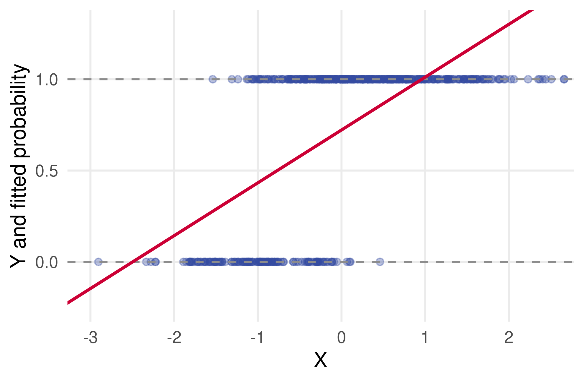
## [1] 0.722

Drawing U \sim \text{Uniform}(0, 1) and setting Y = \mathbf{1}\{U \le p\} gives \mathbf{P}(Y = 1 \mid X) = p exactly.

The true probability is an S-shaped function of X: below 0.02 for X < -2, above 0.97 for X > 0.5.

The linear probability model leaves the unit interval

lpm <- lm(Y ~ X)
coef(lpm)

## (Intercept)           X 
##   0.7220579   0.2893704

mean(fitted(lpm) < 0 | fitted(lpm) > 1)

## [1] 0.17

• The fitted line must keep rising, so 17% of the fitted values fall outside [0, 1].
• A single slope of 0.29 cannot track a curve that is flat in both tails and steep in between.

A link function keeps predictions inside [0, 1]

A generalized linear model (GLM) keeps the linear index X'\beta but passes it through a mean function G:

\mathbf{E}[Y \mid X] = G(X'\beta), \qquad G: \mathbb{R} \to [0, 1].

The usual choice for binary Y is the logistic function

G(z) = \frac{\exp(z)}{1 + \exp(z)} = \frac{1}{1 + \exp(-z)}.

It is increasing, symmetric around G(0) = 0.5, and never reaches 0 or 1.

Strictly, the link is G^{-1}, which maps the mean back to the index; we work with G because it is what produces predictions.

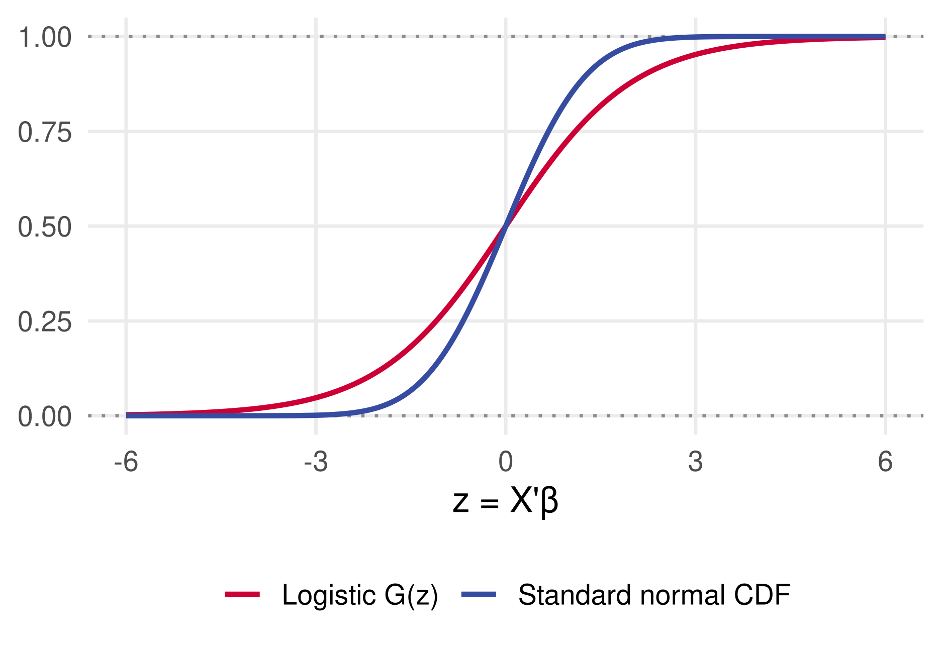
Choosing the normal CDF for G gives the probit model. Its coefficients live on a different scale (appendix).

Logistic regression in one line of R

The GLM with the logistic link is the logistic regression model, or logit:

\mathbf{P}(Y = 1 \mid X) = \frac{\exp(X'\beta)}{1 + \exp(X'\beta)}.

logit_sim <- glm(Y ~ X, family = "binomial")
coef(logit_sim)

## (Intercept)           X 
##    2.184580    3.140629

• The estimates are close to the true values (2, 3) used in the simulation.
• family = "binomial" selects the logistic link by default. Last time we called glm() with its default Gaussian family, which reproduces OLS.
• plogis() computes G in R, and qlogis() its inverse.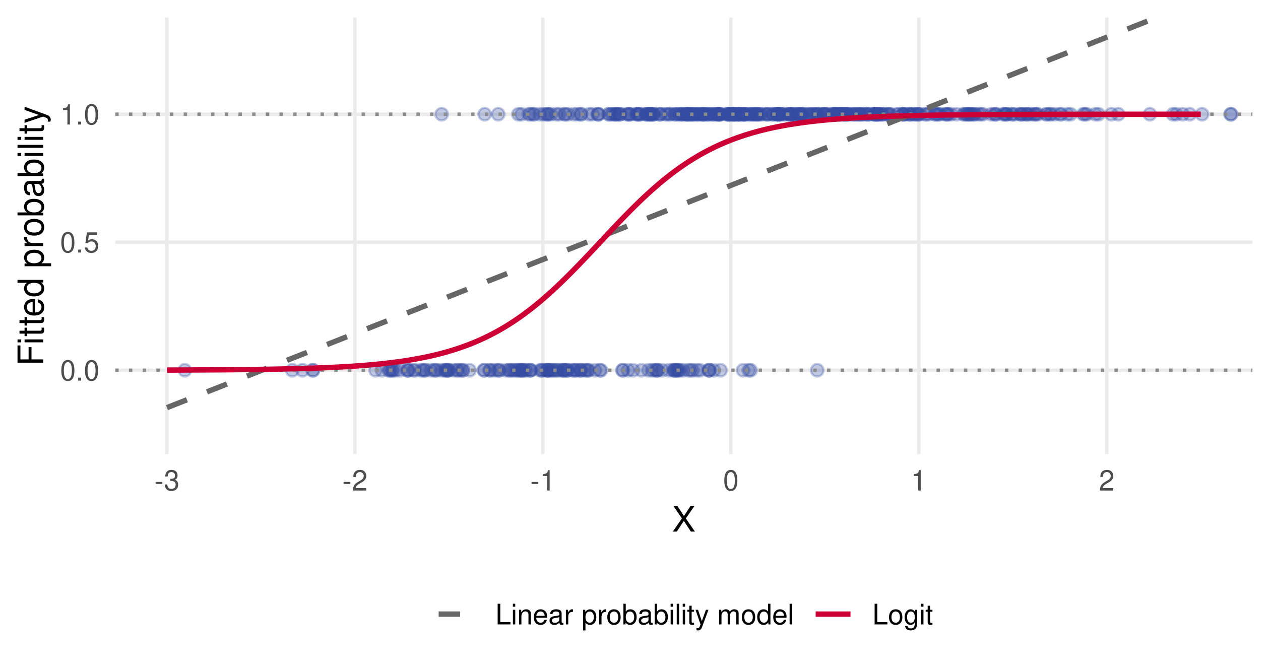

The fitted curve respects the bounds

Both models use the same right-hand side, ~ X. The logit’s predictions approach 0 and 1 smoothly; the LPM line crosses both bounds.

One framework, many outcomes

Outcome	Family in glm()	Mean function G (inverse link)	glm() link g = G^{-1}	Model
Continuous	gaussian (default)	identity, G(z) = z	identity	OLS
Binary	binomial	logistic CDF	logit	Logit
Binary	binomial(link = "probit")	normal CDF \Phi	probit	Probit
Count	poisson	exponential e^z	log	Poisson regression

A GLM has three parts: a distribution for Y, the linear index X'\beta, and the mean function G with \mathbf{E}[Y \mid X] = G(X'\beta). R names each family by the link g = G^{-1}, which maps the mean back to the index; for Poisson, G = \exp and the link is \log.

glm() fits all of them with the same formula interface, so everything we learned about formulas, factors and interactions in the linear regression lecture carries over.

[Sources] - https://www.statmethods.net/advstats/glm.html - https://stat.ethz.ch/R-manual/R-devel/library/stats/html/family.html The appendix gives the exponential dispersion family view and compares probit and logit on the simulated data.

Where the logit comes from: random utility

An agent chooses option 1 over option 0 when its utility is higher. Write the utility difference as

U_1 - U_0 = X'\beta + \varepsilon,

with X'\beta the systematic part and \varepsilon everything the econometrician does not observe. Then

\mathbf{P}(Y = 1 \mid X) = \mathbf{P}(\varepsilon > -X'\beta \mid X) = 1 - F(-X'\beta) = F(X'\beta),

where F is the CDF of \varepsilon and the last step uses symmetry of F around zero.

Distribution of \varepsilon	Model
Logistic	Logit, F(z) = \exp(z)/(1 + \exp(z))
Standard normal	Probit, F(z) = \Phi(z)

\beta measures how X shifts the relative utility of the two options. The same idea extends to several alternatives (multinomial logit) and underlies structural models in IO, labor and public economics.

The scale of epsilon is not identified: multiplying U1 - U0 by a constant leaves the choice unchanged. Logit normalizes the variance to pi^2/3 and probit to 1, which is why logit coefficients are larger by a factor of roughly 1.6 to 1.8 for the same data.

The logit is linear in the log-odds

Since p = e^{z}/(1 + e^{z}) implies 1 - p = 1/(1 + e^{z}), the ratio p/(1 - p) = e^{z}. With z = X'\beta,

\log\left(\frac{\mathbf{P}(Y = 1 \mid X)}{\mathbf{P}(Y = 0 \mid X)}\right) = X'\beta = \beta_1 X_1 + \dots + \beta_d X_d.

The ratio \mathbf{P}(Y = 1 \mid X) / \mathbf{P}(Y = 0 \mid X) is the odds of Y = 1.

Probability	Odds	Log-odds
0.25	1/3	-1.10
0.50	1	0
0.75	3	1.10
0.90	9	2.20

The logit is a linear regression for the log-odds. That is what makes its coefficients interpretable.

Two ways to read a coefficient

Odds. A one-unit increase in X_j multiplies the odds by \exp(\beta_j), a percentage change of

\big(\exp(\beta_j) - 1\big) \times 100\%,

the same arithmetic as for a logged outcome in linear regression, applied to the odds instead of Y. This effect is the same for every observation.

Probability. The slope of \mathbf{P}(Y = 1 \mid X = x) with respect to x_j is the marginal effect

\frac{\partial\, G(x'\beta)}{\partial x_j} = \beta_j\, G(x'\beta)\,\big(1 - G(x'\beta)\big),

which depends on where x is: largest when G(x'\beta) = 0.5, near zero in the tails.

Marginal effects depend on the starting point

b <- coef(logit_sim)
tibble(x = c(-1.5, -1, -0.5, 1)) %>%
  mutate(p = plogis(b[1] + b[2] * x),
         marginal_effect = b[2] * p * (1 - p)) %>%
  knitr::kable(digits = 3)

x	p	marginal_effect
-1.5	0.074	0.215
-1.0	0.278	0.630
-0.5	0.649	0.716
1.0	0.995	0.015

The average marginal effect over the sample is 0.298, close to the LPM slope of 0.289: the LPM can approximate the average effect well even when its individual predictions are poor (code in the appendix).

Checkpoint: interpret the coefficient

A logit for loan repayment gives \hat\beta_{\text{income}} = 0.7 per $10,000 of annual income.

1. By what percentage do the odds of repayment rise per $10,000?
2. For a borrower with \hat p = 0.5, what is the marginal effect on the repayment probability? And at \hat p = 0.9?
3. Why can the same \hat\beta imply different probability changes for different borrowers?

Answers: exp(0.7) - 1 = 1.01, roughly a doubling of the odds; 0.7 x 0.5 x 0.5 = 0.175, and 0.7 x 0.9 x 0.1 = 0.063; the logistic curve is flat in the tails, so the same shift of the index moves the probability less when it is already near 0 or 1.

Likelihood, deviance and fit

---

What glm() maximizes, and how to read its output

Deviance is the fit criterion for OLS

OLS minimizes the sum of squared residuals, which summary() of a Gaussian glm() reports as the residual deviance:

\text{deviance} = \sum_{i=1}^n (Y_i - X_i'\hat\beta)^2.

The null deviance is the same quantity for a model with only an intercept. Since \hat\alpha = \bar Y minimizes \sum_i (Y_i - \alpha)^2,

\text{null deviance} = \sum_{i=1}^n (Y_i - \bar Y)^2.

These are the familiar pieces of the R^2:

R^2 = 1 - \frac{\text{deviance}}{\text{null deviance}} = 1 - \frac{\text{sum of squared residuals}}{\text{total sum of squares}}.

Fit in sample and out of sample

• R^2 = 1 when the residual deviance is 0; R^2 = 0 when the covariates do no better than \bar Y.
• The orange juice regression with brand we talked about last time , price and feature interactions has a null deviance of 30079 and a residual deviance of 13975 (a Gaussian glm() reports both in summary()), so R^2 = (30079 - 13975)/30079 = 0.54. Unobserved factors still drive much of the variation in weekly sales.
• Deviance and R^2 are in-sample measures: the same Y_i are used to fit the model and to evaluate it.
• For prediction we care about out-of-sample fit on new data. In-sample fit can be a poor guide to it; lecture 12 takes this up.

Deviance is what OLS minimizes and how we measure its fit. To fit the logit we need the general version of the same idea: the likelihood.

The deviances quoted are from the model log(sales) ~ log(price) * brand * feat (null 30078.7, residual 13974.8). The baseline model log(sales) ~ log(price) + brand has residual deviance 18224.8 and R-squared 0.39.

The likelihood of the observed data

The likelihood is the probability of the outcomes we observed, under the model, given the covariates. With independent observations \{(y_i, x_i)\}_{i=1}^n,

\mathbf{P}(Y_1 = y_1, \dots, Y_n = y_n \mid X_1 = x_1, \dots, X_n = x_n) = \prod_{i=1}^n \mathbf{P}(Y_i = y_i \mid X_i = x_i).

• For a continuous outcome, replace each probability by the conditional density.
• The likelihood is a function of the parameters with the data held fixed. Maximum likelihood picks the parameter values that make the observed data most probable.
• Logs turn the product into a sum, which is easier to differentiate and to compute without underflow.

Gaussian regression: maximum likelihood is OLS

Take Y_i \mid X_i \sim \mathcal{N}(X_i'\beta, \sigma^2), equivalently Y_i = X_i'\beta + \varepsilon_i with \varepsilon_i \mid X_i \sim \mathcal{N}(0, \sigma^2). The likelihood is

\prod_{i=1}^n \phi(y_i;\, x_i'\beta, \sigma^2) = (2\pi\sigma^2)^{-n/2} \exp\left(-\frac{1}{2\sigma^2}\sum_{i=1}^n (y_i - x_i'\beta)^2\right),

so the log-likelihood is

\log L(\beta, \sigma^2) = -\frac{n}{2}\log(2\pi\sigma^2) - \frac{1}{2\sigma^2}\sum_{i=1}^n (y_i - x_i'\beta)^2.

For any \sigma^2, maximizing over \beta means minimizing the deviance. OLS is the maximum likelihood estimator of the Gaussian linear model: likelihood and deviance are mirror images.

The logit likelihood

Write p_i(\beta) = \mathbf{P}(Y_i = 1 \mid X_i = x_i) = \exp(x_i'\beta)/(1 + \exp(x_i'\beta)). Observation i contributes p_i if y_i = 1 and 1 - p_i if y_i = 0:

L(\beta) = \prod_{i=1}^n p_i(\beta)^{y_i}\,\big(1 - p_i(\beta)\big)^{1 - y_i}.

Taking logs, and using \log p_i = x_i'\beta - \log(1 + e^{x_i'\beta}) and \log(1 - p_i) = -\log(1 + e^{x_i'\beta}),

\log L(\beta) = \sum_{i=1}^n \Big[ y_i\, x_i'\beta - \log\big(1 + \exp(x_i'\beta)\big) \Big].

No closed-form maximizer exists. glm() climbs to \hat\beta by iteratively reweighted least squares, which is the “Fisher Scoring iterations” line at the end of summary().

Derivation check: y log p + (1 - y) log(1 - p) = y[x’b - log(1 + e^{x’b})] - (1 - y) log(1 + e^{x’b}) = y x’b - log(1 + e^{x’b}). Each iteration of IRLS solves a weighted least squares problem with weights p(1 - p), so the logit is computed by repeated OLS.

Each observation votes with its predicted probability

sim %>%
  mutate(p_hat = fitted(logit_sim),
         contribution = if_else(Y == 1, p_hat, 1 - p_hat)) %>%
  slice(1:3) %>%
  knitr::kable(digits = 3)

X	Y	p_hat	contribution
1.263	1	0.998	0.998
-0.326	1	0.761	0.761
1.330	1	0.998	0.998

Each observation contributes the predicted probability of what actually happened: \hat p_i when y_i = 1 and 1 - \hat p_i when y_i = 0. A perfect fit would give every contribution 1, and likelihood 1.

p_hat <- fitted(logit_sim)
c(sum_of_logs = sum(log(if_else(Y == 1, p_hat, 1 - p_hat))),
  logLik = as.numeric(logLik(logit_sim)))

## sum_of_logs      logLik 
##   -151.3337   -151.3337

The log-likelihood has a single peak

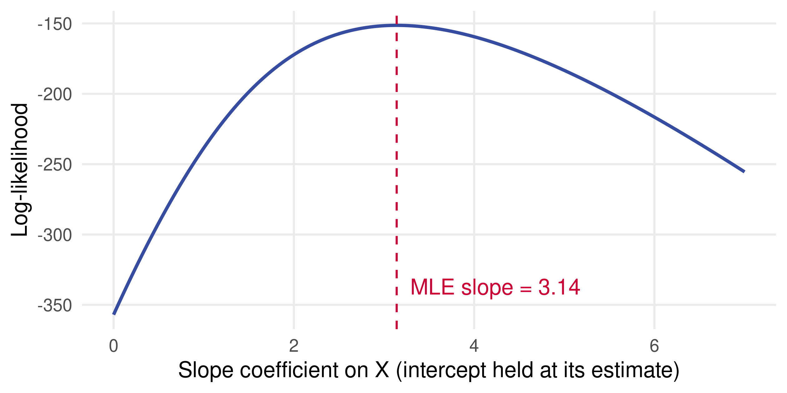
• The logit log-likelihood is concave in \beta, so the iterative search cannot stop at a local maximum: the peak is the glm() estimate.
• The curvature at the peak is the information about \beta; a sharper peak means a smaller standard error.

Deviance for likelihood models

For any likelihood model define

\text{deviance} = -2 \log L(\hat\beta).

• A perfect fit has likelihood 1, so deviance 0. Smaller is better, as with the sum of squared residuals.
• summary() calls this the residual deviance. The null deviance is -2\log L for the intercept-only model, whose fitted probability is \bar Y for everyone.
• R^2 = 1 - \text{deviance}/\text{null deviance} carries over: 1 is a perfect fit, 0 is no improvement on the constant.

round(c(deviance = logit_sim$deviance,
        minus_2_loglik = -2 * as.numeric(logLik(logit_sim)),
        null_deviance = logit_sim$null.deviance,
        R2 = 1 - logit_sim$deviance / logit_sim$null.deviance), 3)

##       deviance minus_2_loglik  null_deviance             R2 
##        302.667        302.667        591.054          0.488

In general the deviance is 2 x (saturated log-likelihood - model log-likelihood). For binary outcomes the saturated model fits every y_i exactly and has log-likelihood 0, so the deviance equals -2 log L. For the Gaussian family glm() reports the sum of squared residuals, which is the deviance up to the sigma^2 scale.

From probabilities to decisions

---

A probability becomes a classification only after we choose a threshold

A threshold turns probabilities into predictions

The logit gives \hat p(x) = \widehat{\mathbf{P}}(Y = 1 \mid X = x). A classifier commits to a label:

\hat Y = \mathbf{1}\{\hat p(X) > t\}.

Which t? Choose it to minimize the expected prediction error

EPE = \mathbf{E}\big[L(Y, \hat Y)\big],

where the loss L(Y, \hat Y) says how bad it is to predict \hat Y when the truth is Y:

\begin{bmatrix} L(0,0) & L(0,1) \\ L(1,0) & L(1,1) \end{bmatrix} = \begin{bmatrix} 0 & L(0,1) \\ L(1,0) & 0 \end{bmatrix}.

L(0,1) is the cost of a false positive (predict 1, truth 0) and L(1,0) the cost of a false negative. Correct guesses cost nothing.

The Bayes rule and the cost-ratio threshold

Condition on X = x and write p(x) = \mathbf{P}(Y = 1 \mid X = x). The expected loss of each decision is

\hat Y = 1: \; L(0,1)\,\big(1 - p(x)\big), \qquad \hat Y = 0: \; L(1,0)\, p(x).

The Bayes classifier picks the cheaper one:

\hat Y_{\text{Bayes}}(x) = \mathbf{1}\big\{L(1,0)\, p(x) > L(0,1)\,\big(1 - p(x)\big)\big\} = \mathbf{1}\left\{p(x) > \frac{L(0,1)}{L(0,1) + L(1,0)}\right\}.

Loss	Threshold
0-1 loss, L(0,1) = L(1,0) = 1	t = 0.5: predict the more probable class
False positive twice as costly as false negative	t = 2/3
False negative twice as costly as false positive	t = 1/3

In practice we plug in \hat p(x) from the logit. The threshold encodes the relative costs of the two mistakes.

[Sources] - Hastie, Tibshirani and Friedman (2009), The Elements of Statistical Learning, section 2.4. With 0-1 loss the Bayes rule is the mode of the conditional distribution, argmax_k P(Y = k | X = x), which is the form given in the notes.

Four numbers summarize a classifier

For a given threshold, cross-tabulate truth against prediction:

	Predicted 0	Predicted 1
Actual 0	true negatives (TN)	false positives (FP)
Actual 1	false negatives (FN)	true positives (TP)

Measure	Definition	Question it answers
Accuracy	(TP + TN)/n	How often is the label right?
Sensitivity (recall)	TP/(TP + FN)	Share of actual positives we catch
Specificity	TN/(TN + FP)	Share of actual negatives we clear
Precision	TP/(TP + FP)	Share of flagged cases that are right

Sensitivity estimates \mathbf{P}(\hat Y = 1 \mid Y = 1) and specificity \mathbf{P}(\hat Y = 0 \mid Y = 0). Accuracy flatters a model when one class dominates: predicting the majority class for everyone already scores its share.

The ROC curve traces every threshold

Lowering t raises sensitivity and lowers specificity. The receiver operating characteristic (ROC) curve plots the pairs

\big(1 - \text{specificity},\ \text{sensitivity}\big)

as t moves from 1 down to 0.

• Each point on the curve is one confusion matrix.
• The diagonal is random guessing: predicting 1 with probability q regardless of x gives sensitivity q and false positive rate q.
• The top-left corner is a perfect classifier.

AUC: the area under the ROC curve

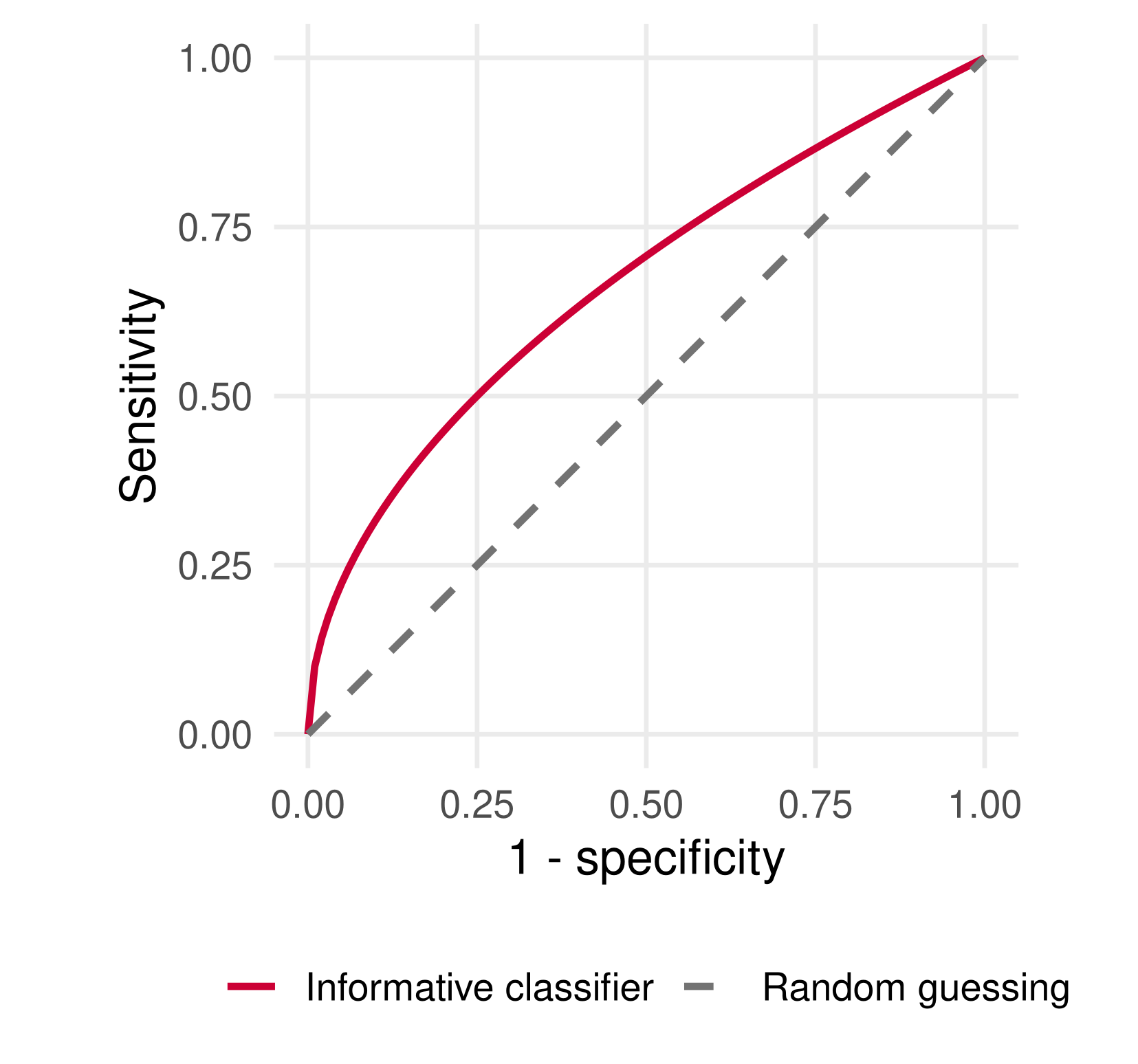
The AUC compresses the curve into one number.

• \text{AUC} = \mathbf{P}\big(\hat p(X_1) > \hat p(X_0)\big) for a randomly drawn positive X_1 and a randomly drawn negative X_0: the probability that the model ranks a random positive above a random negative.
• 0.5 is uninformative and 1 is a perfect ranking.
• It does not depend on any threshold, so it evaluates the probabilities themselves rather than one decision rule.

Use the AUC to compare models. Use the cost ratio to choose the threshold you deploy.

[Sources] - Fawcett (2006), An introduction to ROC analysis, Pattern Recognition Letters 27, 861-874. The probabilistic interpretation is the Wilcoxon-Mann-Whitney statistic; ties between a positive and a negative score count one half.

Checkpoint: moving the threshold

A hospital screens patients for a disease with a logit and a threshold t.

1. If missing a case is far costlier than a false alarm, should t move up or down?
2. What happens to sensitivity and specificity as t falls toward 0?
3. Two models have the same AUC. Can they still produce different numbers of false positives at t = 0.5?

Answers: down, since a large L(1,0) pushes L(0,1)/(L(0,1) + L(1,0)) toward 0; sensitivity rises to 1 and specificity falls to 0 because every patient is flagged; yes, the AUC summarizes the ranking, while the count of false positives at a fixed threshold depends on the level of the predicted probabilities.

A spam filter

---

Your inbox runs a logistic regression

The spam data

Y_i = 1 if a human labeled email i as spam, 0 otherwise. X_i describes the email: 48 word indicators, 6 character indicators and 3 measures of capital-letter runs.

email <- read.csv("data/spam.csv")
dim(email)

## [1] 4601   58

email[1:3, c("word_free", "word_george", "char_dollar",
             "capital_run_length_total", "spam")]

##   word_free word_george char_dollar capital_run_length_total spam
## 1         1           0           0                      278    1
## 2         1           0           1                     1028    1
## 3         1           0           1                     2259    1

table(email$spam)

## 
##    0    1 
## 2788 1813

Emails 1, \dots, n have been labeled by a person. The task: predict whether a new email is spam from its features.

[Sources] - https://archive.ics.uci.edu/dataset/94/spambase This version of the UCI Spambase data records each word and character as a 0/1 indicator rather than the original percentage frequencies; the three capital-run-length variables keep their original scale.

Fit the logit with every feature

logit <- glm(spam ~ ., data = email, family = "binomial")
round(coef(summary(logit))[c("word_free", "word_george", "word_hp",
                             "char_dollar", "char_exclaim"), ], 3)

##              Estimate Std. Error z value Pr(>|z|)
## word_free       1.543      0.179   8.621        0
## word_george    -5.780      0.758  -7.623        0
## word_hp        -3.604      0.387  -9.316        0
## char_dollar     1.871      0.207   9.016        0
## char_exclaim    1.343      0.146   9.220        0

• ~ . puts every other column of the data set on the right-hand side, so the model has 57 slope coefficients. summary(logit) prints them all; the table shows five.
• The signs already tell a story: free, $ and ! raise the log-odds of spam, while george and hp lower them.
• The z value column is the estimate divided by its standard error

Read a coefficient as a percentage change in odds

(exp(coef(logit)[c("word_george", "word_free")]) - 1) * 100

## word_george   word_free 
##   -99.69108   367.72294

• An email containing “george” has odds of being spam 99.7% lower than an otherwise identical email without it.
• Containing “free” raises the odds of spam by 368%, holding the other 56 features fixed.

Cross-check against the raw counts:

table(spam = email$spam, george = email$word_george)

##     george
## spam    0    1
##    0 2016  772
##    1 1805    8

Only 8 of the 1,813 spam emails contain “george”, against 772 of the 2,788 legitimate ones.

The corpus was assembled at Hewlett-Packard Labs in the late 1990s. The legitimate emails came from the work inbox of an HP employee named George, which is why “george”, “hp” and the Palo Alto area code “650” are strong non-spam indicators. Spammers of the time did not personalize their messages.

Predict the probability of spam

predict(logit, newdata = email[c(1, 12), ], type = "response")

##         1        12 
## 0.8839073 0.8772593

email$spam[c(1, 12)]

## [1] 1 1

• type = "response" returns \hat p = G(x'\hat\beta). The default, type = "link", returns the log-odds x'\hat\beta.
• Both emails are predicted spam with probability about 0.88, and both are spam.
• The syntax is the same as for linear regressions: a fitted model plus newdata.

Deviance and R^2 for the spam logit

c(null = logit$null.deviance, residual = logit$deviance,
  minus_2_loglik = -2 * as.numeric(logLik(logit)))

##           null       residual minus_2_loglik 
##       6170.153       1548.660       1548.660

1 - logit$deviance / logit$null.deviance

## [1] 0.7490079

• summary(logit) reports the same two deviances at the bottom of its output.
• The 57 features explain about three quarters of the deviance of spam status. A perfect classifier would drive the residual deviance to 0.
• As for OLS, this is an in-sample fit.

Classify at the 0.5 threshold

spam_probs <- predict(logit, type = "response")
spam_pred <- as.integer(spam_probs > 0.5)
confusion <- table(Actual = email$spam, Predicted = spam_pred)
confusion

##       Predicted
## Actual    0    1
##      0 2669  119
##      1  167 1646

tibble(accuracy = sum(diag(confusion)) / sum(confusion),
       sensitivity = confusion[2, 2] / sum(confusion[2, ]),
       specificity = confusion[1, 1] / sum(confusion[1, ]),
       precision = confusion[2, 2] / sum(confusion[, 2])) %>%
  knitr::kable(digits = 3)

accuracy	sensitivity	specificity	precision
0.938	0.908	0.957	0.933

The filter catches 91% of spam and wrongly flags 4% of legitimate mail, in sample.

Move the threshold, move the trade-off

classify <- function(t, y = email$spam, p = spam_probs) {
  yhat <- as.integer(p > t)
  tibble(threshold = t, sensitivity = mean(yhat[y == 1] == 1),
         specificity = mean(yhat[y == 0] == 0), accuracy = mean(yhat == y))
}
map_dfr(c(0.1, 0.3, 0.5, 0.7, 0.9), classify) %>% knitr::kable(digits = 3)

threshold	sensitivity	specificity	accuracy
0.1	0.990	0.761	0.851
0.3	0.949	0.915	0.928
0.5	0.908	0.957	0.938
0.7	0.846	0.976	0.925
0.9	0.702	0.991	0.877

A legitimate email lost in the spam folder usually costs more than a spam email that gets through, so a provider might set t above 0.5: at t = 0.9 only 1% of legitimate mail is flagged, while 30% of spam gets through.

The ROC curve is the threshold table drawn out

thresholds <- round(seq(0, 1, by = 0.005), 3)
roc_hand <- map_dfr(thresholds, classify)
marks <- roc_hand %>%
  filter(threshold %in% c(0.1, 0.5, 0.9))

• Every row of roc_hand is one confusion matrix.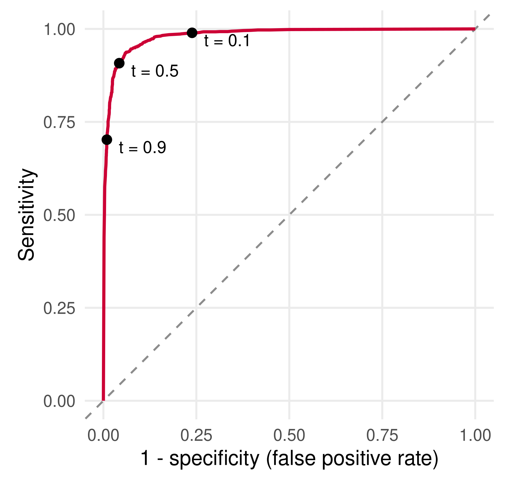
• The three labelled points are rows of the table on the previous slide.
• Moving from t = 0.9 to t = 0.1 walks up and to the right along the curve.

pROC computes the curve and the area

roc_spam <- roc(email$spam, spam_probs, quiet = TRUE)
auc(roc_spam)

## Area under the curve: 0.9825

• roc() evaluates every distinct threshold in the predicted probabilities; coords(roc_spam, "all") returns the same sensitivity and specificity pairs we computed by hand, and plot(roc_spam) draws the curve.
• An AUC of 0.98 means the model ranks a randomly chosen spam email above a randomly chosen legitimate one 98% of the time.
• The AUC is a property of the ranking. Which threshold to deploy is still the cost question from the previous slide.

[Sources] - https://cran.r-project.org/package=pROC roc() prints a message about the direction of the comparison unless quiet = TRUE; the direction is inferred from the data, so check it when the labels are unusual.

Hotel reviews

---

Predicting a high rating from the adjectives a review uses

Ratings and adjective counts for 210,000 reviews

load("data/tripadvisor.RData")
c(train = nrow(X_train), test = nrow(X_test), adjectives = ncol(X_train))

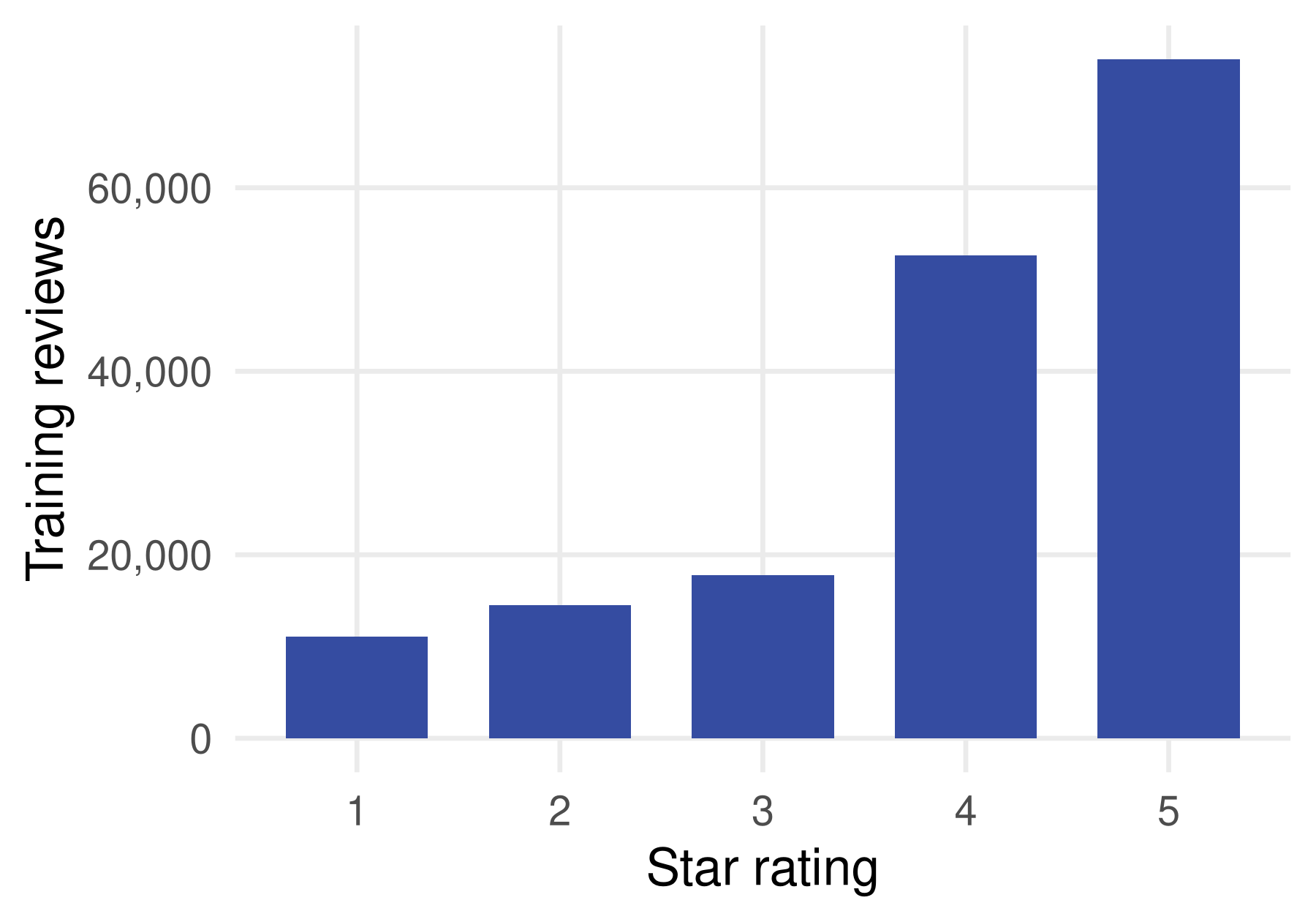
##      train       test adjectives 
##     169987      40000       7573

class(X_train)

## [1] "dgCMatrix"
## attr(,"package")
## [1] "Matrix"

y_train[1:10]

##  [1] 1 5 4 5 4 5 4 5 2 5

• Each row is a TripAdvisor hotel review: y is its 1 to 5 star rating and X counts how many times the review uses each of 7,573 adjectives.
• The data come already split into 169,987 training reviews and 40,000 test reviews.

[Sources] - https://github.com/yanxht/TripAdvisorData - Wang, Lu and Zhai (2010), KDD; Yan and Bien (2021), JASA. The reviews were collected by Wang, Lu and Zhai and processed into adjective counts by Yan and Bien for their work on rare features.

The counts are stored as a sparse matrix

X_train[1:6, 1:5]

## 6 x 5 sparse Matrix of class "dgCMatrix"
##     Terms
## Docs arrogant decided large minor beat
##    1        1       .     .     .    .
##    2        .       .     .     .    .
##    3        .       .     .     .    .
##    4        .       1     3     .    .
##    5        .       .     1     1    .
##    6        .       .     .     .    .

nnzero(X_train) / prod(dim(X_train))     # share of nonzero entries

## [1] 0.003047276

format(object.size(X_train), "Mb")

## [1] "55.8 Mb"

• Dots are zeros. Only 0.3% of the entries are nonzero, so the dgCMatrix format from lecture 8 stores the whole matrix in 56 MB.
• A dense copy would need 169987 \times 7573 \times 8 bytes, about 9.6 GB.

Most reviews are positive

mean(y_train >= 4)

## [1] 0.7448452

• Our outcome is whether a review gives 4 or 5 stars: Y_i = \mathbf{1}\{\text{rating}_i \ge 4\}.
• Three quarters of the training reviews are positive, so a classifier that says “4+” for everyone is already right 74% of the time. Any model has to beat that.

Most adjectives are rare

uses_per_review <- Matrix::colMeans(X_train)   # average number of uses per review
head(sort(uses_per_review, decreasing = TRUE), 6)

##     great      good       one      nice      just     clean 
## 0.9082459 0.6806815 0.5764323 0.5167630 0.4968086 0.3836058

mean(uses_per_review < 0.01)

## [1] 0.9429552

• “great” is used 0.9 times per review on average (it appears in 48% of reviews). The median adjective appears in fewer than one review in 10,000.
• 94% of the adjectives average fewer than one use per 100 reviews. Such columns carry little information and make the design matrix large.

Matrix::colMeans on the count matrix gives the mean number of uses per review, not the share of reviews containing the word; “great” appears in 48% of reviews although its mean count is 0.91 because some reviews use it several times. The 0.05 cutoff below follows the notes so that the 123-word model and its coefficients match.

Keep the adjectives that are used often enough

keep <- which(uses_per_review > 0.05)
length(keep)

## [1] 123

X_train_kept <- as.matrix(X_train[, keep])   # dense, 123 columns
format(object.size(X_train_kept), "Mb")

## [1] "169.9 Mb"

• The rule keeps 123 adjectives averaging more than one use per 20 reviews: great, clean, friendly, disappointed and so on.
• The dense matrix of 123 kept columns takes three times the memory of the sparse matrix with all 7,573 columns. Sparse storage is a decision about zeros, not about size.
• glm() needs an ordinary data frame, which is why we convert after pruning.

Build the training and test sets, then fit

dat_train <- as_tibble(X_train_kept) %>% mutate(is_4or5 = y_train >= 4)
dat_test <- as_tibble(as.matrix(X_test[, keep])) %>% mutate(is_4or5 = y_test >= 4)
hotel_model <- glm(is_4or5 ~ ., family = "binomial", data = dat_train)

• The outcome is whether the review gives 4 or 5 stars; the predictors are the 123 adjective counts.
• The same keep columns are used for the 40,000 test reviews, which play no role in estimation.
• Fitting 124 coefficients on 169,987 reviews takes a few seconds. summary(hotel_model) prints 124 rows, so we look at the extremes instead.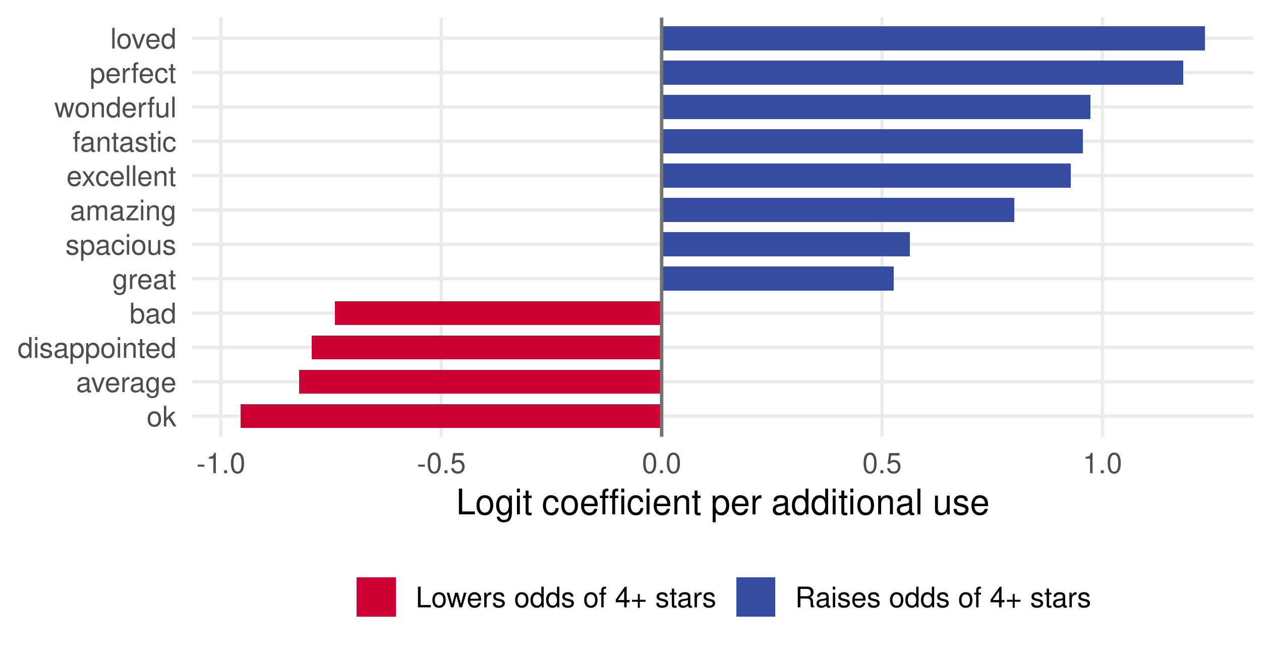

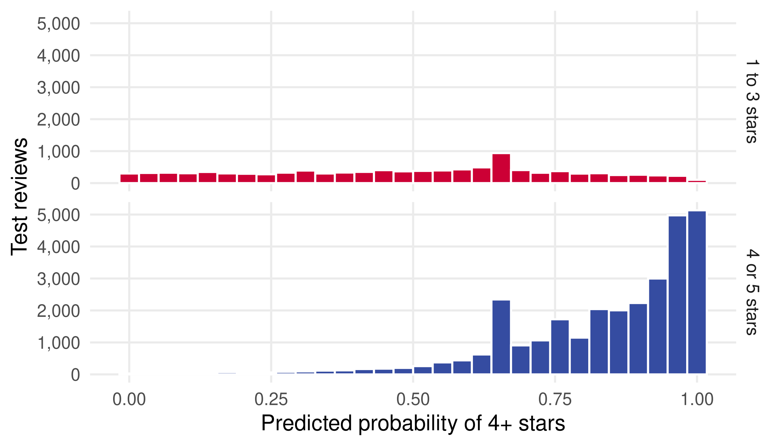
The largest coefficients make sense

coef_tbl %>% slice_head(n = 12)   # the same numbers as a table

Enthusiastic words raise the log-odds; lukewarm words such as “ok” and “average” lower them as much as “bad” does.

Odds multipliers for single words

exp(coef(hotel_model)[c("fantastic", "ok")])

## fantastic        ok 
## 2.6017806 0.3846518

• Each additional use of “fantastic” multiplies the odds of a 4+ rating by 2.6, an increase of 160%, holding the other 122 counts fixed.
• Each use of “ok” multiplies the odds by 0.38, a decrease of 62%.
• The multipliers compound: two uses of “fantastic” and one of “ok” give 2.6^2 \times 0.38 \approx 2.6.

Out-of-sample predictions separate the classes

pred_test <- predict(hotel_model, newdata = dat_test, type = "response")
tapply(pred_test, dat_test$is_4or5, median)

##     FALSE      TRUE 
## 0.5226444 0.8874854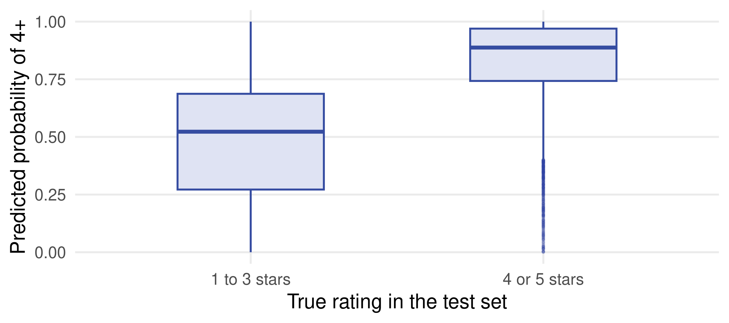

Reviews that really are 4+ get a median predicted probability of 0.89, the rest 0.52. The classes overlap, so no threshold separates them perfectly.

ROC and AUC on the test set

roc_test <- roc(dat_test$is_4or5, pred_test, quiet = TRUE)
roc_train <- roc(dat_train$is_4or5, fitted(hotel_model),
                 quiet = TRUE)
c(train = as.numeric(auc(roc_train)),
  test = as.numeric(auc(roc_test)))

##     train      test 
## 0.8625054 0.8584706

c(accuracy_at_0.5 = mean((pred_test > 0.5) == dat_test$is_4or5),
  always_4plus = mean(dat_test$is_4or5))

## accuracy_at_0.5    always_4plus 
##        0.830125        0.741075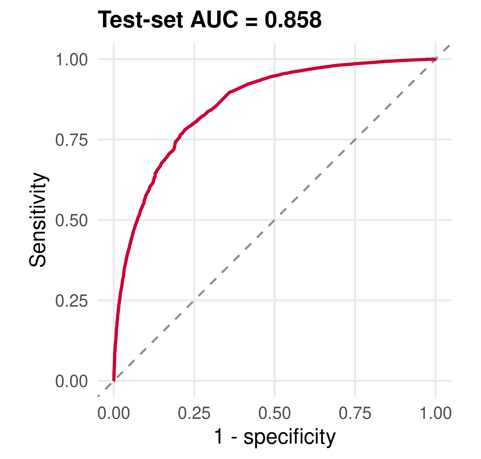

• Training and test AUC are almost equal: with 124 coefficients and 170,000 reviews there is little room to overfit.
• At t = 0.5 the model is right 83% of the time on new reviews, against 74% for always predicting 4+.

Checkpoint: the modelling choices

1. Why report the AUC on the 40,000 test reviews rather than on the 169,987 training reviews?
2. What would change if we kept every adjective averaging at least one use per 100 reviews (432 of them) instead of 123?
3. A review uses “fantastic” twice and “ok” once. By what factor do its odds of 4+ stars change relative to a review using neither?

Answers: the training fit is optimistic because the same reviews chose the coefficients, here only mildly so; more columns, a slower fit, coefficients on rare words with larger standard errors, and a test AUC that may rise or fall, which is the variable-selection question lecture 13 addresses; 2.6^2 x 0.38, about 2.6, so the odds still rise by a factor of roughly 2.6.

Ranking from pairwise comparisons

---

The Bradley-Terry model is a logit in disguise

A model for who beats whom

Teams, players, products or chatbots meet in pairs, and we observe who wins. The Bradley-Terry model gives each competitor i a rating \beta_i and sets

\log \frac{\mathbf{P}(i \text{ beats } j)}{1 - \mathbf{P}(i \text{ beats } j)} = \beta_i - \beta_j, \qquad\text{so}\qquad \mathbf{P}(i \text{ beats } j) = \frac{e^{\beta_i - \beta_j}}{1 + e^{\beta_i - \beta_j}} = \frac{e^{\beta_i}}{e^{\beta_i} + e^{\beta_j}}.

• Only differences in ratings matter. Equal ratings give a coin flip; a gap of 1 gives the stronger side a 73% chance.
• The goal is to estimate the ratings from match outcomes and rank the competitors, as the Elo system does in chess.
• The basic model has no ties. The appendix records a tie as half a win for each side.

[Sources] - Bradley and Terry (1952), Biometrika 39, 324-345. Elo updates a rating after every game with a fixed step; Bradley-Terry fits all games at once by maximum likelihood, which is why leaderboards moved to it.

It is a logistic regression with a special design matrix

Index each match by the pair (i, j) and occasion t, with m competitors in total:

• y_{ijt} = \mathbf{1}\{i \text{ beats } j \text{ at } t\};
• x_{ijt} = e_i - e_j \in \mathbb{R}^m, where e_i is the i-th unit vector.

Then x_{ijt}'\beta = \beta_i - \beta_j, and the model reads \text{logit}\,\mathbf{P}(y_{ijt} = 1) = x_{ijt}'\beta: a logit with no intercept.

Match	y	A	B	C
A vs B, A wins	1	1	-1	0
B vs C, C wins	0	0	1	-1
A vs C, A wins	1	1	0	-1
C vs B, C wins	1	0	-1	1

Stacking the n matches gives y \in \mathbb{R}^n and X \in \mathbb{R}^{n \times m} with one +1 and one -1 in each row.

Ratings are identified only up to a constant

Adding the same constant to every \beta_i leaves every difference \beta_i - \beta_j, and so every probability, unchanged. Each row of X sums to zero, so X has rank at most m - 1.

Fix the level by setting \beta_m = 0 for one reference competitor. Dropping column m,

X\beta = X_{-m}\beta_{-m}, \qquad \beta_{-m} \in \mathbb{R}^{m - 1},

and the MLE over \beta_{-m} is the constrained MLE. Every other rating is then measured relative to competitor m.

Extensions fit in the same regression:

• an intercept captures an advantage shared by whoever is listed first, such as home field;
• match covariates (altitude, rest days, prompt type) enter as extra columns;
• a tie can be recorded as half a win and half a loss (appendix).

Pairwise comparisons train today’s language models

In reinforcement learning from human feedback (RLHF), annotators compare two responses to the same prompt and pick the better one.

• A reward model r(\cdot) is trained so that the Bradley-Terry probability of the preferred response, G\big(r(\text{A}) - r(\text{B})\big), is high: the reward plays the role of the rating.
• The language model is then tuned to produce responses with high reward, and the cycle repeats.

We turn the idea around: instead of scoring responses, rate the models themselves from head-to-head battles.

[Sources] - https://arxiv.org/abs/2203.02155 (Ouyang et al. 2022, InstructGPT) - https://arxiv.org/abs/2411.04991 (Sun, Shen and Ton 2024) The reward-model loss in InstructGPT is the negative log of the Bradley-Terry probability of the preferred response. Sun, Shen and Ton examine when the Bradley-Terry assumption is appropriate for reward modelling and discuss alternatives.

Chatbot Arena: humans vote, models compete

• A user enters a prompt, sees two anonymous responses from different models, and votes for the better one or a tie.
• The public leaderboard ranks models with a Bradley-Terry model fitted to the accumulated votes.
• We use a released sample of 57,477 battles among 64 models.

[Sources] - https://arxiv.org/abs/2403.04132 (Chiang et al. 2024) - https://lmsys.org/blog/2023-12-07-leaderboard/ - https://huggingface.co/datasets/lmarena-ai/arena-human-preference-55k The screenshot is a saved snapshot; the live page at lmarena.ai/leaderboard changes continuously. The December 2023 blog post explains the switch from online Elo updates to a Bradley-Terry fit with bootstrap confidence intervals.

Read only the columns we need

dat <- read_csv("data/train_small.csv", show_col_types = FALSE,
                col_select = c(model_a, model_b, winner_model_a,
                               winner_model_b, winner_tie))
dim(dat)

## [1] 57477     5

head(dat, 4)

## # A tibble: 4 × 5
##   model_a            model_b             winner_model_a winner_model_b winner_tie
##   <chr>              <chr>                        <dbl>          <dbl>      <dbl>
## 1 gpt-4-1106-preview gpt-4-0613                       1              0          0
## 2 koala-13b          gpt-4-0613                       0              1          0
## 3 gpt-3.5-turbo-0613 mistral-medium                   0              0          1
## 4 llama-2-13b-chat   mistral-7b-instruct              1              0          0

col_select skips the prompt and response text, so the 184 MB file loads in a fraction of a second. Each row is one battle: the two models, and which one the user preferred.

Outcomes and appearances

dat %>% summarize(a_wins = mean(winner_model_a), b_wins = mean(winner_model_b),
                  ties = mean(winner_tie))

## # A tibble: 1 × 3
##   a_wins b_wins  ties
##    <dbl>  <dbl> <dbl>
## 1  0.349  0.342 0.309

appearances <- bind_rows(
  dat %>% transmute(model = model_a, win = winner_model_a, tie = winner_tie),
  dat %>% transmute(model = model_b, win = winner_model_b, tie = winner_tie))
appearances %>% count(model, sort = TRUE) %>% head(4)

## # A tibble: 4 × 2
##   model                  n
##   <chr>              <int>
## 1 gpt-4-1106-preview  7387
## 2 gpt-3.5-turbo-0613  7083
## 3 gpt-4-0613          6165
## 4 claude-2.1          5583

Wins split evenly between the two positions and 31% of battles end in a tie. Appearances per model range from 100 to more than 7,000.

Raw win rates are a tempting shortcut

raw <- appearances %>%
  filter(tie == 0) %>%
  group_by(model) %>%
  summarize(battles = n(), win_rate = mean(win)) %>%
  arrange(desc(win_rate))
head(raw, 6)

## # A tibble: 6 × 3
##   model              battles win_rate
##   <chr>                <int>    <dbl>
## 1 gpt-4-1106-preview    5360    0.760
## 2 gpt-4-0125-preview     798    0.747
## 3 gpt-3.5-turbo-0314     968    0.735
## 4 gpt-4-0314            2923    0.682
## 5 claude-1              2792    0.626
## 6 qwen1.5-72b-chat       370    0.581

• gpt-3.5-turbo-0314 sits third with a 73.5% win rate. Did it face the same opponents as the GPT-4 models?
• A win rate ignores who was beaten. The Bradley-Terry model conditions on the opponent in every match.

Build the design matrix

models <- sort(unique(c(dat$model_a, dat$model_b)))
dat_noties <- dat %>%
  filter(winner_tie == 0) %>%
  mutate(model_a = factor(model_a, levels = models),
         model_b = factor(model_b, levels = models))
x <- model.matrix(~ model_a - 1, data = dat_noties) -
     model.matrix(~ model_b - 1, data = dat_noties)
colnames(x) <- str_remove(colnames(x), "^model_a")
dat_noties[1:2, 1:2]

## # A tibble: 2 × 2
##   model_a            model_b   
##   <fct>              <fct>     
## 1 gpt-4-1106-preview gpt-4-0613
## 2 koala-13b          gpt-4-0613

x[1:2, c("gpt-4-1106-preview", "gpt-4-0613", "koala-13b")]

##   gpt-4-1106-preview gpt-4-0613 koala-13b
## 1                  1         -1         0
## 2                  0         -1         1

model.matrix(~ model_a - 1) gives one indicator column per model, the vector e_i; subtracting the model_b version gives e_i - e_j. Shared levels keep the 64 columns aligned.

Fit the model with glm()

baseline <- colnames(x)[ncol(x)]
x <- x[, -ncol(x)]                      # drop one column: its rating is 0
bt <- glm(dat_noties$winner_model_a ~ x - 1, family = "binomial")
ratings <- tibble(model = c(str_remove(names(coef(bt)), "^x"), baseline),
                  rating = c(coef(bt), 0)) %>%
  arrange(desc(rating)) %>%
  mutate(bt_rank = row_number())
head(ratings, 6)

## # A tibble: 6 × 3
##   model              rating bt_rank
##   <chr>               <dbl>   <int>
## 1 gpt-4-0125-preview  1.76        1
## 2 gpt-4-1106-preview  1.73        2
## 3 gpt-4-0314          1.11        3
## 4 gpt-4-0613          0.954       4
## 5 qwen1.5-72b-chat    0.897       5
## 6 mistral-medium      0.861       6

• - 1 removes the intercept, and the dropped reference model (zephyr-7b-beta) has rating 0 by construction.
• The GPT-4 versions lead, followed by qwen1.5-72b-chat and mistral-medium.

The rating adjusts for the strength of the schedule

compare %>%
  filter(model %in% c("gpt-4-1106-preview", "gpt-3.5-turbo-0314",
                      "claude-2.1", "koala-13b")) %>%
  select(model, battles, win_rate, raw_rank, rating, bt_rank, opponent_rating) %>%
  knitr::kable(digits = 2)

model	battles	win_rate	raw_rank	rating	bt_rank	opponent_rating
gpt-4-1106-preview	5360	0.76	1	1.73	2	0.54
claude-2.1	3969	0.43	36	0.57	13	0.87
gpt-3.5-turbo-0314	968	0.73	3	0.43	22	-0.76
koala-13b	1102	0.51	20	-0.54	52	-0.58

• gpt-3.5-turbo-0314 drops from 3rd to 22nd: its opponents were the weakest in the data, with an average rating of -0.76.
• claude-2.1 rises from 36th to 13th: it was matched mostly against strong models.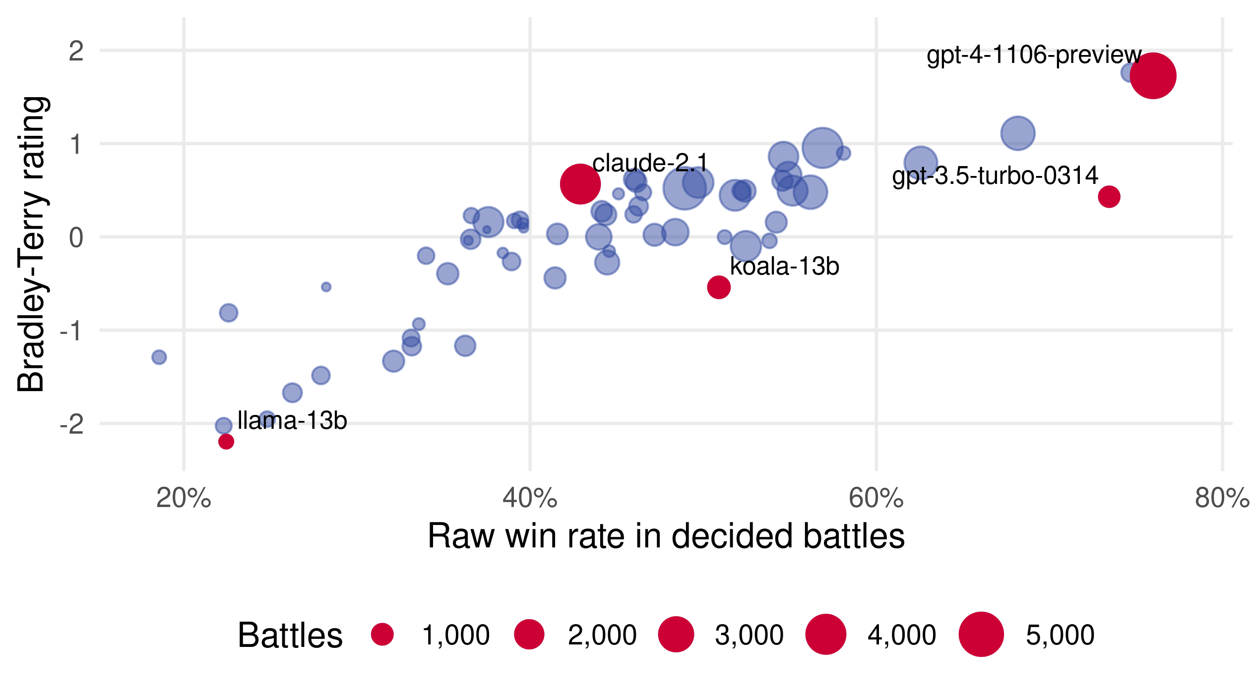

Ratings against win rates

The two measures agree broadly, but models that met weak opponents sit below the cloud and models that met strong ones sit above it.

From ratings to predicted win probabilities

beta_hat <- setNames(ratings$rating, ratings$model)
top3 <- ratings$model[1:3]
round(outer(beta_hat[top3], beta_hat[top3], function(bi, bj) plogis(bi - bj)), 2)

##                    gpt-4-0125-preview gpt-4-1106-preview gpt-4-0314
## gpt-4-0125-preview               0.50               0.51       0.66
## gpt-4-1106-preview               0.49               0.50       0.65
## gpt-4-0314                       0.34               0.35       0.50

plogis(beta_hat["gpt-4-1106-preview"] - beta_hat["gpt-3.5-turbo-0613"])

## gpt-4-1106-preview 
##          0.7696009

• Entry (i, j) is the predicted probability that the row model beats the column model. The two GPT-4 Turbo previews are a coin flip against each other and beat gpt-4-0314 about two thirds of the time.
• Against gpt-3.5-turbo-0613, gpt-4-1106-preview is predicted to win 77% of decided battles.

Refinements used by the live leaderboard

bt_int <- glm(dat_noties$winner_model_a ~ x, family = "binomial")
round(coef(summary(bt_int))["(Intercept)", ], 3)

##   Estimate Std. Error    z value   Pr(>|z|) 
##      0.025      0.011      2.303      0.021

• The intercept estimates a first-position advantage. Model A’s log-odds are 0.025 higher, small but statistically detectable. Responses are shown side by side, so position could matter.
• The leaderboard treats ties as half wins (appendix) and reports bootstrap confidence intervals for the ratings (next time).
• The rating scale is arbitrary. Chatbot Arena reports 1000 + 400\,\hat\beta_i/\log 10, the Elo convention, so a 400-point gap corresponds to 10-to-1 odds:

round(1000 + 400 * beta_hat[top3] / log(10))

## gpt-4-0125-preview gpt-4-1106-preview         gpt-4-0314 
##               1306               1300               1193

[Sources] - https://lmsys.org/blog/2023-12-07-leaderboard/ - https://colab.research.google.com/drive/1KdwokPjirkTmpO_P1WByFNFiqxWQquwH The leaderboard notebook fits the logistic regression on the design matrix scaled by log(10) and reports 400 x coefficient + 1000, which is the Elo scale: P(i beats j) = 1 / (1 + 10^(-(R_i - R_j)/400)). Ties are entered twice, once as a win for each side, with weight one half each.

Practice: rate the models yourself

1. Refit the Bradley-Terry model with gpt-4-0613 as the reference model (rating 0). Which ratings change, and which predicted probabilities?
2. Add the intercept. Does the ranking of the top five change?
3. Include the tied battles as half wins (appendix code). Compare the top ten with and without ties.
4. Using ratings, compute the probability that claude-2.1 beats mixtral-8x7b-instruct-v0.1.

Answers: every rating shifts by the same constant, so all differences and probabilities are unchanged; the intercept is common to all matches and leaves the ranking of the top five unchanged in these data; the tie-inclusive ratings are compressed toward zero but the ordering is almost identical (correlation 0.999 with the no-tie fit); plogis of the rating difference.

The logit in one page

A binary outcome is a probability model. The logit keeps the linear index X'\beta and maps it into [0, 1]; coefficients act on the log-odds.

Likelihood generalizes least squares. OLS is the Gaussian MLE, the logit maximizes the Bernoulli likelihood, and deviance = -2\log L replaces the sum of squared residuals.

Probabilities become decisions through a threshold. The threshold encodes the cost ratio; the ROC curve and the AUC evaluate the ranking without one.

The same glm() call scales from 2 to 124 coefficients. Sparse storage, a held-out test set and an out-of-sample AUC keep large problems honest.

Pairwise comparisons are a logit with a special design. The Bradley-Terry model turns match outcomes into ratings, from chess to chatbots.

Reading and data sources

• James, Witten, Hastie and Tibshirani, An Introduction to Statistical Learning, chapter 4: logistic regression and classification.
• Hastie, Tibshirani and Friedman, The Elements of Statistical Learning, section 2.4: expected prediction error and the Bayes classifier.
• Bradley and Terry (1952): the paired-comparison model; Sun, Shen and Ton (2024): Bradley-Terry in reward modelling.
• Chiang et al. (2024) and the LMSYS leaderboard post: Chatbot Arena and its ratings; battle data.
• Wang, Lu and Zhai (2010) and Yan and Bien (2021): the TripAdvisor review data, from this repository.
• UCI Spambase: the spam data. Package references: pROC, GLM families in R.

Additional derivations and code

---

Optional material for reference and practice

GLMs and the exponential dispersion family

The classical linear model “Y \sim \mathcal{N}(X'\beta, \sigma^2)” bundles three choices: a random component Y \sim \mathcal{N}(\mu, \sigma^2), a systematic component \eta = X'\beta, and the link \mu = \eta.

A GLM changes the first and the third:

1. Y follows an exponential dispersion family density f(y; \theta, \phi) = \exp\left[\frac{y\theta - b(\theta)}{a(\phi)} + c(y, \phi)\right], with natural parameter \theta and dispersion \phi. The normal, the Bernoulli and binomial, and the Poisson are all members.
2. The mean is linked to the index by \mathbf{E}[Y] = g^{-1}(X'\beta); in the lecture’s notation G = g^{-1}.

For the Bernoulli, \theta = \log\frac{\mu}{1 - \mu} is the log-odds, so the logit is the canonical link: the natural parameter itself is linear in X. Likelihood computations and inference stay tractable across the whole family.

Bernoulli check: mu^y (1 - mu)^(1 - y) = exp(y log(mu / (1 - mu)) + log(1 - mu)), so theta = logit(mu), b(theta) = log(1 + e^theta), a(phi) = 1 and c = 0.

Probit and logit on the simulated data

probit_sim <- glm(Y ~ X, family = binomial(link = "probit"))
rbind(logit = coef(logit_sim), probit = coef(probit_sim),
      ratio = coef(logit_sim) / coef(probit_sim))

##        (Intercept)        X
## logit     2.184580 3.140629
## probit    1.253479 1.813304
## ratio     1.742814 1.731993

max(abs(fitted(logit_sim) - fitted(probit_sim)))

## [1] 0.01556418

• Coefficients are not comparable across links: the logistic distribution has standard deviation \pi/\sqrt{3} \approx 1.8 against 1 for the standard normal, so logit coefficients are larger by a factor of about 1.6 to 1.8.
• The fitted probabilities are nearly identical. Compare marginal effects and predictions across links, not raw coefficients.

Average marginal effects in R

me <- function(model, var) {
  p <- fitted(model)
  coef(model)[var] * p * (1 - p)             # logit: dG/dz = G(1 - G)
}
c(average_marginal_effect = mean(me(logit_sim, "X")),
  lpm_slope = unname(coef(lpm)["X"]))

## average_marginal_effect               lpm_slope 
##               0.2975717               0.2893704

For a binary regressor, report the average discrete change instead: predict with the indicator switched on and off for every observation and average the difference.

email_1 <- email_0 <- email
email_1$word_free <- 1
email_0$word_free <- 0
mean(predict(logit, newdata = email_1, type = "response") -
     predict(logit, newdata = email_0, type = "response"))

## [1] 0.09421097

Switching “free” on raises the predicted probability of spam by 9.4 percentage points on average.

Test-set predictions by class

Ties as half wins in the Bradley-Terry model

ties <- dat %>%
  filter(winner_tie == 1) %>%
  mutate(model_a = factor(model_a, levels = models),
         model_b = factor(model_b, levels = models))
x_tie <- model.matrix(~ model_a - 1, data = ties) - model.matrix(~ model_b - 1, data = ties)
colnames(x_tie) <- str_remove(colnames(x_tie), "^model_a")
x_tie <- x_tie[, colnames(x)]
X_all <- rbind(x, x_tie, x_tie)              # each tie enters twice ...
y_all <- c(dat_noties$winner_model_a, rep(1, nrow(ties)), rep(0, nrow(ties)))
w_all <- c(rep(1, nrow(x)), rep(0.5, 2 * nrow(ties)))   # ... with weight one half
bt_ties <- glm(y_all ~ X_all - 1, family = "binomial", weights = w_all)

A tie is entered as a win and a loss for the first model, each with weight one half. The likelihood then counts half a win and half a loss for every tied battle.

glm() warns about non-integer successes when the weights are fractional; the estimates are still the weighted maximum likelihood estimates, and family = quasibinomial gives identical coefficients without the warning.

Ties compress the ratings but keep the order

ratings_ties <- tibble(model = c(str_remove(names(coef(bt_ties)), "^X_all"), baseline),
                       rating = c(coef(bt_ties), 0)) %>%
  arrange(desc(rating))
head(ratings_ties, 5)

## # A tibble: 5 × 2
##   model              rating
##   <chr>               <dbl>
## 1 gpt-4-1106-preview  1.20 
## 2 gpt-4-0125-preview  1.19 
## 3 gpt-4-0314          0.780
## 4 gpt-4-0613          0.674
## 5 qwen1.5-72b-chat    0.605

cor(ratings_ties$rating, ratings$rating[match(ratings_ties$model, ratings$model)])

## [1] 0.9992817

• Every tie is evidence that the two models are close, so the ratings shrink toward zero: the leader’s rating falls from 1.76 to 1.20.
• The ordering is essentially unchanged, and the top two swap places by a hair.

Install the required packages

Run once in your R environment if needed:

install.packages(c("tidyverse", "Matrix", "pROC"))

Data files, all read from lectures/data/:

• spam.csv, a 0/1 version of the UCI Spambase data;
• tripadvisor.RData, from github.com/yanxht/TripAdvisorData;
• train_small.csv, the training file of the Chatbot Arena human preference data.

Every example in this deck runs offline once the files are in place.

Return to the question

Is the outcome a probability? Then model the log-odds, maximize the likelihood, and decide with a threshold that reflects the costs.

Return to the main takeaway