ECON 4370 / 6370 Computing for Economics

Lecture 8: Linear Regression

Zhan Gao

24 September 2026

Three questions, one tool

Question Outcome Y Covariates X
How much do orange-juice sales fall when the price rises? log sales log price, brand, promotion
What is a one-bedroom condo in Los Angeles worth? price size, bathrooms, location
How much does a household spend online? log spending broadband access

Regression estimates how the average outcome varies with covariates. Today’s tool is the linear model, fitted with lm() or glm().

Today’s route

  1. Prediction as a conditional expectation: define the target.
  2. The linear model and OLS: approximate the target with a line.
  3. Orange juice: dummies, logs, and interactions.
  4. Housing: confounding, multicollinearity, and heterogeneity.

Robust standard errors and other details follow the main lesson.

Packages and data

Run the examples from the lectures/ directory.

library(tidyverse)
library(patchwork)   # side-by-side plots
Data Unit Used for
data/web-browsers.csv 10,000 households, one year of online spending Conditional distributions
data/oj.csv Store-week-brand sales at 83 Dominick’s stores Demand elasticities
data/redfinLA3.csv 133 one-bedroom condo listings in Los Angeles Confounding and interactions

The appendix also uses sandwich and lmtest. Plots use three SMU colours stored in smu_colors.

Prediction as a conditional expectation


Define the target before estimating anything

Supervised learning has an outcome

Each observation carries an outcome Y and covariates X.

Setting Outcome Method
Regression Continuous Y Linear regression (today)
Classification Discrete Y, often 0 or 1 Logistic regression (next lecture)
Unsupervised learning No Y Learn structure in X (later)

The goal is to learn the relationship between X and Y from a sample, then predict Y' for new units with covariates X'.

To make “prediction” precise, we use conditional expectations.

The target is a conditional mean

\mathbf{E}[Y \mid X = x] is the average outcome in the population among units with covariates x.

Written as \mathbf{E}[Y \mid X], it is a function of X: one prediction for every value of the covariates.

Why the mean rather than the exact value?

  • We observe only a few of the factors that influence Y. Given that limitation, we make the best prediction we can.
  • The conditional distribution \mathbf{P}(Y = y \mid X = x) carries more information, but the mean is a convenient summary of its centre.

Regression estimates \mathbf{E}[Y \mid X]. Everything else today is a choice about how to approximate it.

The sample analogue is a cell mean

Average the outcomes of the sampled units that share the covariate value x:

\hat{\mathbf{E}}[Y \mid X = x] = \frac{\sum_{i=1}^n Y_i\,\mathbf{1}\{X_i = x\}}{\sum_{i=1}^n \mathbf{1}\{X_i = x\}}.

This works when X takes a few values, so that every cell holds many observations.

We will see shortly why it breaks down with continuous or many covariates.

Online spending: the marginal distribution

browser <- read.csv("./data/web-browsers.csv")
dim(browser)
## [1] 10000     7
p_spend <- ggplot(browser, aes(x = log(spend))) +
  geom_histogram(bins = 30, fill = smu_blue,
                 colour = "white") +
  geom_vline(xintercept = mean(log(browser$spend)),
             colour = smu_red, linewidth = 1) +
  labs(x = "log(spend)", y = "Households")

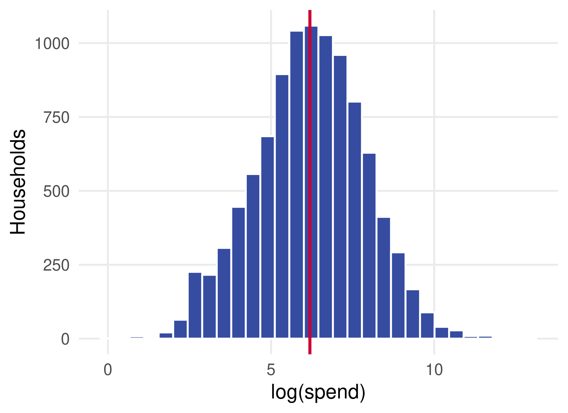
The histogram uses no covariate. The red line is the unconditional sample mean of log spending.

Histogram of log annual online spending for 10,000 households, roughly bell shaped, with a vertical red line at the sample mean.

Condition on broadband access

p_box <- ggplot(browser,
    aes(x = factor(broadband), y = log(spend),
        fill = factor(broadband))) +
  geom_boxplot(show.legend = FALSE) +
  scale_fill_manual(values = smu_colors) +
  labs(x = "Broadband access", y = "log(spend)")
browser %>% group_by(broadband) %>%
  summarise(mean_log_spend = mean(log(spend)),
            n = n())
## # A tibble: 2 × 3
##   broadband mean_log_spend     n
##       <int>          <dbl> <int>
## 1         0           5.73  1749
## 2         1           6.29  8251

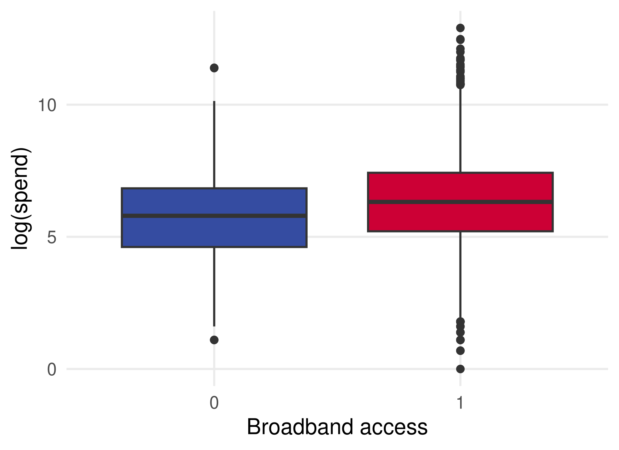
Two boxplots of log spending, for households without and with broadband. The broadband box sits higher, with a higher median and upper quartile.

Each box summarizes a conditional distribution. The group means are the cell-mean estimates of \mathbf{E}[\log(\textit{spend}) \mid \textit{broadband}].

Reading a boxplot

Element Meaning
Thick middle line Median
Box Interquartile range (IQR): first to third quartile
Whiskers Most extreme points within 1.5 IQR of the box
Dots beyond the whiskers Outliers

Households with broadband spend more on average, and the whole distribution shifts up, not only its centre.

Checkpoint: sample or population?

The histogram, the boxplots and the group means were computed from n = 10{,}000 households.

  1. Are these sample objects or population objects?
  2. What population object does each one estimate?
  3. What would change if we drew a fresh sample of 10,000 households?

The linear model and OLS


A line as an approximation to the conditional mean

Linear regression assumes a linear conditional mean

\mathbf{E}[Y_i \mid X_i] = X_i'\beta = \beta_1 X_{i1} + \beta_2 X_{i2} + \dots + \beta_d X_{id}.

X_i is a vector of d characteristics and \beta a vector of d coefficients:

X_i = \begin{pmatrix} X_{i1} \\ \vdots \\ X_{id} \end{pmatrix}, \qquad \beta = \begin{pmatrix} \beta_1 \\ \vdots \\ \beta_d \end{pmatrix}.

To include an intercept, set X_{i1} = 1 for every i, so that \beta_1 is the intercept.

“Linear” means linear in \beta. The entries of X_i can be logs, indicators, or products of other variables.

The error form of the same model

Equivalently,

Y_i = X_i'\beta + \varepsilon_i, \qquad \mathbf{E}[\varepsilon_i \mid X_i] = 0.

The error \varepsilon_i collects every determinant of Y_i other than X_i. Taking conditional expectations,

\mathbf{E}[Y_i \mid X_i] = \mathbf{E}[X_i'\beta \mid X_i] + \underbrace{\mathbf{E}[\varepsilon_i \mid X_i]}_{0} = X_i'\beta.

The mean-zero condition says that the covariates carry no information about the average error.

Simulate from a regression model

set.seed(0)
n <- 500
X <- rpois(n, lambda = 1)
eps <- rnorm(n)
Y <- 1 + 3 * X + eps
sim <- data.frame(X, Y)

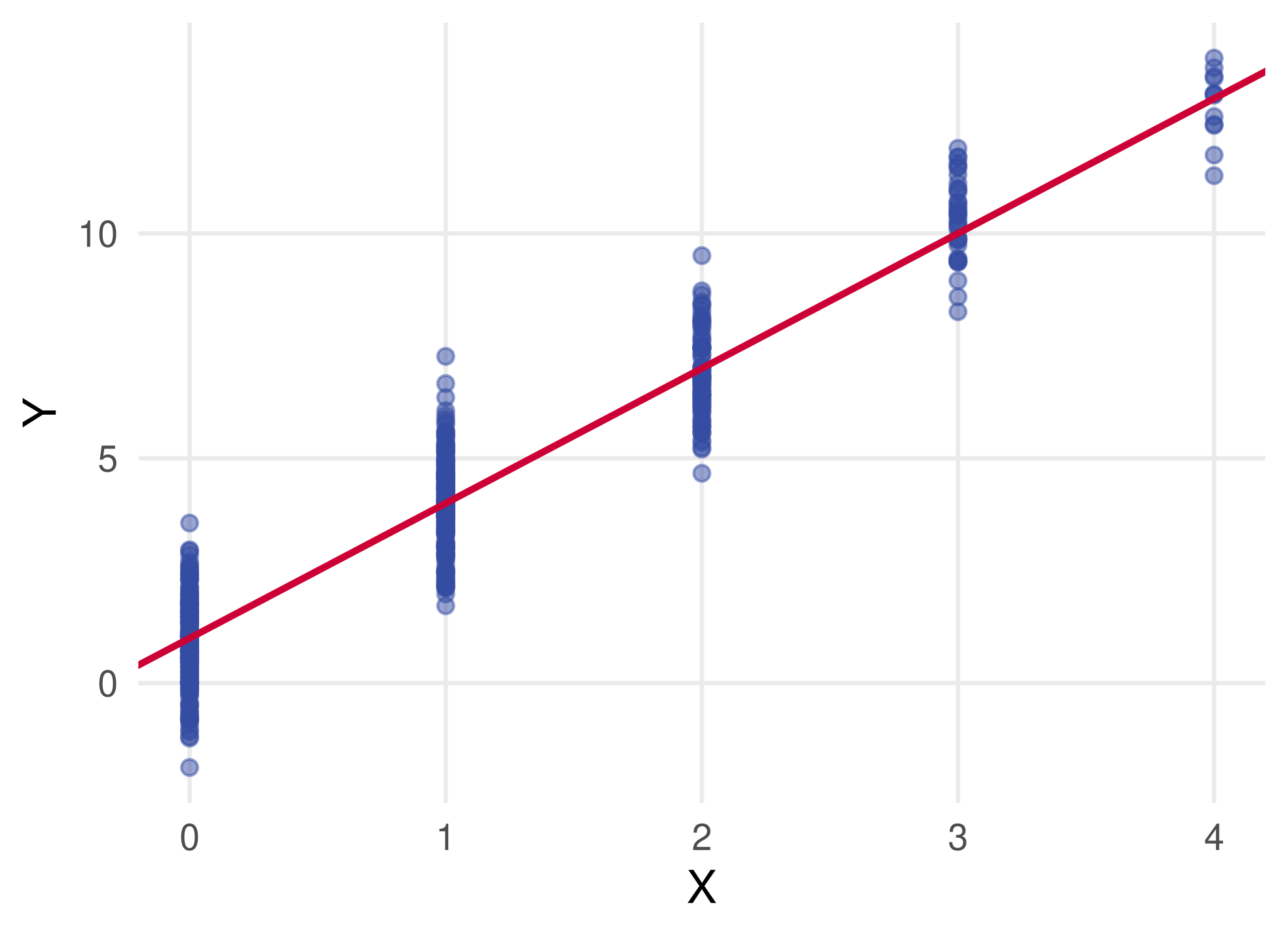
Here \mathbf{E}[Y_i \mid X_i] = 1 + 3X_i by construction.

Increasing X by one unit raises Y by 3 on average. The red line is the conditional mean.

Scatterplot of 500 simulated points with X taking integer values from 0 to 4 and Y scattered around the red line Y equals 1 plus 3X.

Cell means recover the slope, with noise

table(X)
## X
##   0   1   2   3   4 
## 181 193  78  36  12
mean(Y[X == 2]) - mean(Y[X == 1])
## [1] 2.874353

The difference is close to 3 but not equal to it: each cell mean carries sampling error, and the cells with large X are small.

Why cell means do not scale:

  • With a continuous covariate, no two units share exactly the same x. Every cell has one observation.
  • With many covariates, the number of cells explodes and most of them are empty.

A linear model pools information across cells: two parameters instead of one mean per cell.

OLS chooses the best-fitting line

The ordinary least squares (OLS) estimator solves

\min_{b} \sum_{i=1}^n (Y_i - X_i'b)^2.

Each unit contributes its squared approximation error; the minimizer is the best fit in total. The first-order conditions give a closed form involving a matrix inverse:

\hat\beta = \left(\sum_{i=1}^n X_iX_i'\right)^{-1} \sum_{i=1}^n X_iY_i.

coef(lm(Y ~ X, data = sim))
## (Intercept)           X 
##   0.9131373   3.0546537

R’s lm() computes this for us. The appendix shows where the formula comes from.

One formula interface for every model

lm(y ~ x1 + x2, data = df) fits OLS. glm() takes the same formula and, by default, fits the same Gaussian model.

Formula term Meaning
y ~ x Intercept plus a slope on x
y ~ x + z Add a regressor
y ~ log(x) Transform inside the formula
y ~ f, with f a factor One indicator per level, first level omitted
y ~ x * f x, f, and their products x:f
y ~ x - 1 Drop the intercept

Next lecture keeps this interface and changes the family argument of glm().

OLS is also the best linear predictor

We motivated OLS with a linear conditional mean. A second motivation needs no such assumption.

OLS minimizes \frac{1}{n}\sum_{i=1}^n (Y_i - X_i'b)^2, the sample analogue of \mathbf{E}[(Y_i - X_i'b)^2], so it estimates

\beta^{*} = \arg\min_{b}\ \mathbf{E}\left[(Y_i - X_i'b)^2\right],

the population best linear predictor of Y_i given X_i.

  • This interpretation holds even when \mathbf{E}[Y_i \mid X_i] is nonlinear: X_i'\beta^{*} is then the best linear approximation to it.
  • As a prediction rule: given X_{n+1}, predict X_{n+1}'\hat\beta.
  • Neither interpretation makes \hat\beta a causal effect. That requires further assumptions.

One regressor: the slope is a scaled correlation

With X_i = (1, D_i)', the OLS slope is

\hat\beta_2 = \frac{\widehat{\text{Cov}}(Y, D)}{\widehat{\text{Var}}(D)} = \widehat{\text{Corr}}(Y, D)\,\sqrt{\frac{\widehat{\text{Var}}(Y)}{\widehat{\text{Var}}(D)}},

since the sample correlation is \widehat{\text{Cov}}(Y, D)\big/\sqrt{\widehat{\text{Var}}(D)\,\widehat{\text{Var}}(Y)}.

c(slope = cov(Y, X) / var(X), lm = unname(coef(lm(Y ~ X, data = sim))[2]))
##    slope       lm 
## 3.054654 3.054654

OLS repackages a sample correlation. Correlation is not causation.

A binary regressor reproduces the cell means

Regress log spending on the 0/1 broadband indicator:

coef(lm(log(spend) ~ broadband, data = browser))
## (Intercept)   broadband 
##    5.732062    0.555759
browser %>% group_by(broadband) %>% summarise(mean_log_spend = mean(log(spend)))
## # A tibble: 2 × 2
##   broadband mean_log_spend
##       <int>          <dbl>
## 1         0           5.73
## 2         1           6.29

The intercept is the mean for households without broadband. The slope is the difference in means.

With one indicator regressor, OLS is the cell-mean estimator. With continuous regressors, it pools across cells instead.

Checkpoint: from one indicator to many

  1. In lm(log(spend) ~ broadband), what does the intercept estimate?
  2. Suppose a covariate has three categories. How many indicators does a model with an intercept need, and why not three?
  3. Which interpretation of OLS survives if the true conditional mean is a curve?

Orange juice demand


Dummies, logs, and interactions in one dataset

Weekly orange-juice sales at 83 stores

oj <- read.csv("./data/oj.csv")
dim(oj)
## [1] 28947     4
head(oj, 4)
##   sales price     brand feat
## 1  8256  3.87 tropicana    0
## 2  6144  3.87 tropicana    0
## 3  3840  3.87 tropicana    0
## 4  8000  3.87 tropicana    0

One row per brand and store-week.

Variable Meaning
sales Units moved that week
price Price per unit ($)
brand Dominick’s, Minute Maid, or Tropicana
feat 1 if the brand was featured (advertised) in the store that week

Brand is a categorical variable

Store it as a factor so R knows the categories and their order:

oj$brand <- factor(oj$brand)
levels(oj$brand)
## [1] "dominicks"   "minute.maid" "tropicana"
table(oj$brand, oj$feat)
##              
##                  0    1
##   dominicks   7169 2480
##   minute.maid 6865 2784
##   tropicana   8045 1604

The first level, Dominick’s, will be the baseline category in regressions. The three brands have equal numbers of rows, but how often each is featured differs.

Each brand occupies its own price range

p_price <- ggplot(oj,
    aes(x = brand, y = log(price), fill = brand)) +
  geom_boxplot(show.legend = FALSE) +
  scale_fill_manual(values = smu_colors) +
  labs(x = NULL, y = "log(price)")

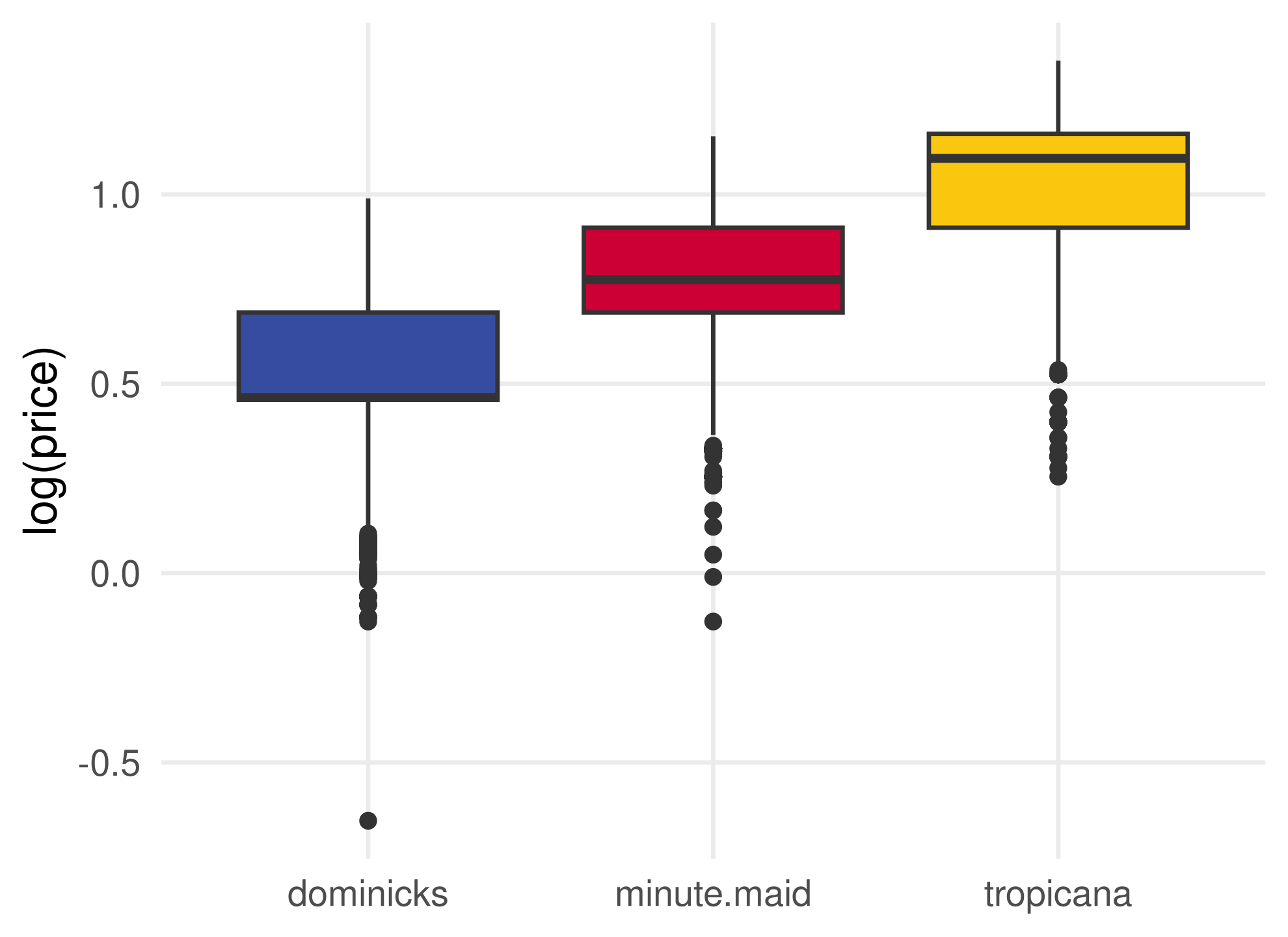
Tropicana is the premium brand, Minute Maid sits in the middle, and Dominick’s is the store brand.

Prices also vary a lot within brand across stores and weeks. That variation identifies the price response.

Boxplots of log price for the three brands. Tropicana has the highest prices, Minute Maid intermediate, and Dominick's the lowest, with overlapping ranges.

Logs straighten the demand curve

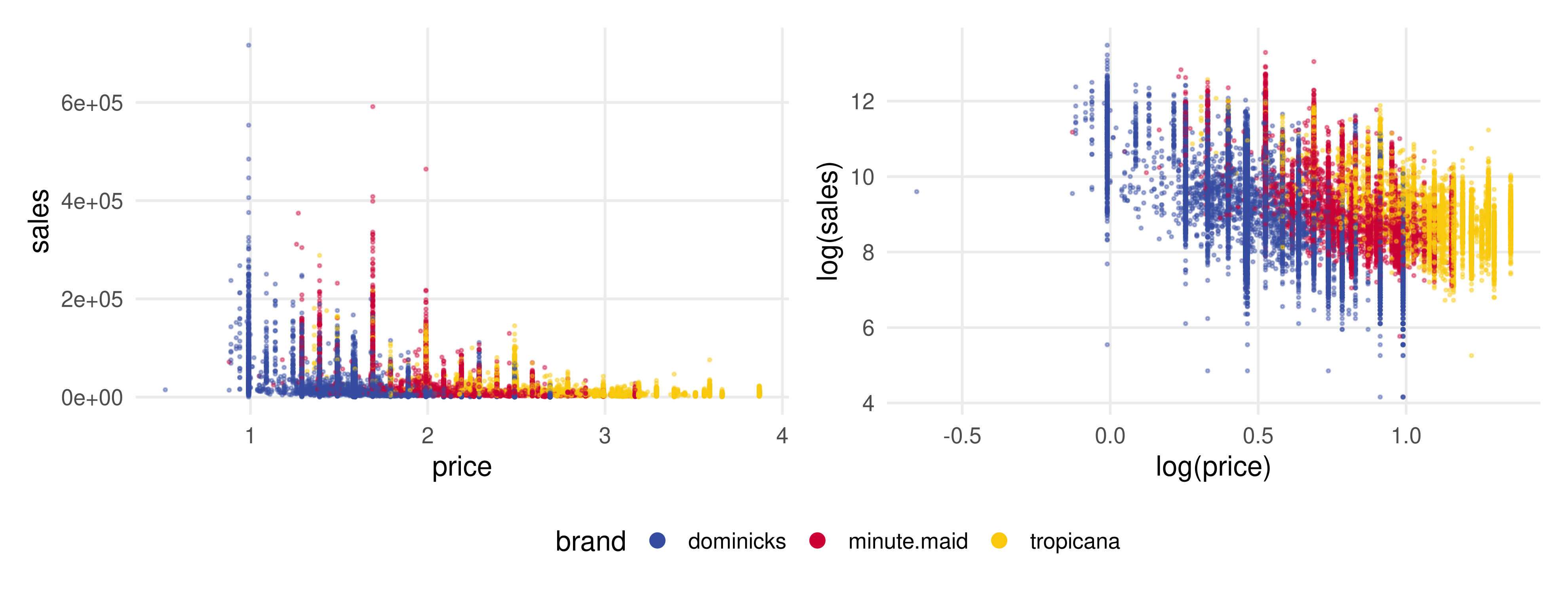
Two scatterplots of the orange-juice data coloured by brand. Left: sales against price on raw scales, with bursts of very high sales at low prices. Right: log sales against log price, where each brand forms a roughly linear, downward-sloping cloud.

Raw scale: occasional bursts of sales at low prices, consistent with stocking up during promotions. Log scale: a roughly linear law of demand, sales fall as price rises.

A regression with brand dummies

On the log scale, fit

\log(\textit{sales}_i) = \beta_1 + \beta_2 \log(\textit{price}_i) + \beta_3\, \textit{minutemaid}_i + \beta_4\, \textit{tropicana}_i + \varepsilon_i,

where \textit{minutemaid}_i = 1 if the row is Minute Maid and 0 otherwise, and similarly for \textit{tropicana}_i.

  • These 0/1 variables are indicator or dummy variables; machine learning calls the construction one-hot encoding.
  • The omitted category, Dominick’s, is the baseline: \beta_3 and \beta_4 are shifts relative to it.
  • One slope \beta_2 applies to all three brands. We relax this soon.

R builds the dummies from the factor

OLS_model <- glm(log(sales) ~ log(price) + brand, data = oj)
head(model.matrix(OLS_model), 4)
##   (Intercept) log(price) brandminute.maid brandtropicana
## 1           1   1.353255                0              1
## 2           1   1.353255                0              1
## 3           1   1.353255                0              1
## 4           1   1.353255                0              1

model.matrix() shows the regressors R actually used: an intercept column, log price, and one indicator per non-baseline brand.

glm() with its default Gaussian family gives the same estimates as lm(). We use it here so that the interface is familiar when the family changes next lecture.

The fitted model

summary(OLS_model)
## 
## Call:
## glm(formula = log(sales) ~ log(price) + brand, data = oj)
## 
## Coefficients:
##                  Estimate Std. Error t value Pr(>|t|)    
## (Intercept)      10.82882    0.01453  745.04   <2e-16 ***
## log(price)       -3.13869    0.02293 -136.89   <2e-16 ***
## brandminute.maid  0.87017    0.01293   67.32   <2e-16 ***
## brandtropicana    1.52994    0.01631   93.81   <2e-16 ***
## ---
## Signif. codes:  0 '***' 0.001 '**' 0.01 '*' 0.05 '.' 0.1 ' ' 1
## 
## (Dispersion parameter for gaussian family taken to be 0.6296804)
## 
##     Null deviance: 30079  on 28946  degrees of freedom
## Residual deviance: 18225  on 28943  degrees of freedom
## AIC: 68765
## 
## Number of Fisher Scoring iterations: 2

Read the coefficients

Term Estimate Interpretation
log(price) -3.14 A 1% higher price goes with about 3.1% lower sales, holding brand fixed
brandminute.maid 0.87 Log sales are 0.87 higher than Dominick’s at the same price
brandtropicana 1.53 Log sales are 1.53 higher than Dominick’s at the same price

The price coefficient in a log-log model is an elasticity.

Every coefficient is a comparison that holds the other regressors fixed. It is not the raw difference between brands in the data.

Interpreting a logged outcome

Model Change in D Change in Y
\log Y on \log D 1% higher D about \beta%, an elasticity
\log Y on continuous D D up by one unit about 100\beta%
\log Y on a 0/1 dummy D D from 0 to 1 (e^{\beta} - 1)\times 100%

The first two rows use the calculus approximation \Delta\log Y \approx \Delta Y / Y, accurate for small changes.

For a dummy, no approximation is needed: \log(Y_1) - \log(Y_0) = \beta gives \dfrac{Y_1 - Y_0}{Y_0} = e^{\beta} - 1.

(exp(coef(OLS_model)["brandtropicana"]) - 1) * 100
## brandtropicana 
##       361.7913

At the same price, Tropicana sells about 362% more units than Dominick’s, not 153% more.

The model imposes parallel slopes

Draw fitted lines by predicting on a grid:

grid <- expand.grid(
  price = seq(min(oj$price), max(oj$price),
              length.out = 100),
  brand = levels(oj$brand))
grid$fit <- predict(OLS_model, newdata = grid)
p_par <- ggplot(oj,
    aes(log(price), log(sales), colour = brand)) +
  geom_point(size = 0.3, alpha = 0.25) +
  geom_line(data = grid, aes(y = fit),
            linewidth = 1.1) +
  scale_colour_manual(values = smu_colors) +
  labs(x = "log(price)", y = "log(sales)")

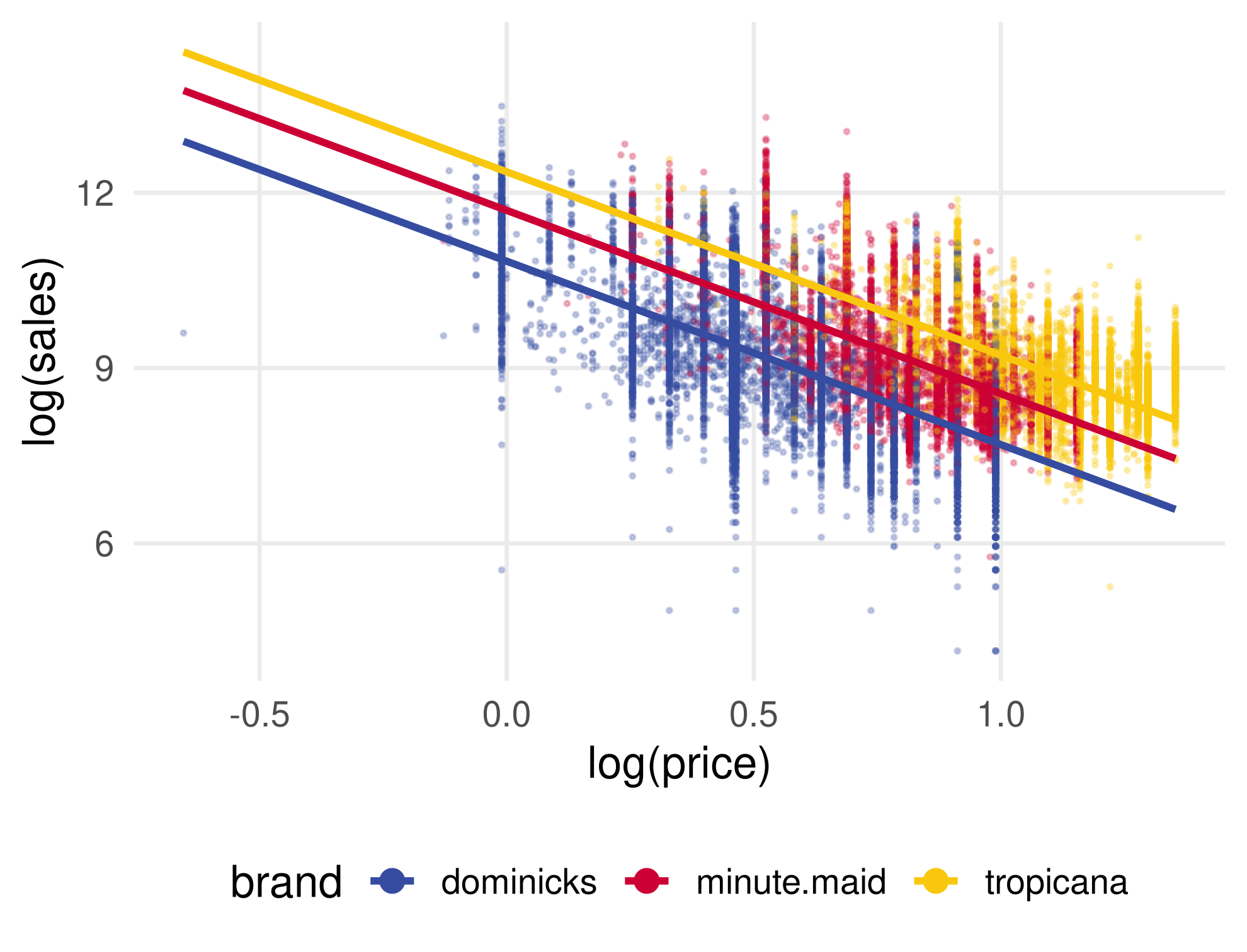
Scatterplot of log sales against log price by brand with three parallel fitted lines, one per brand, from the model without interactions.

Brands shift the line up or down. The slope, the price elasticity, is forced to be the same.

Interactions let the slope differ by brand

Customers of a premium brand may be less price sensitive. That is a difference in slopes, not in levels.

\begin{aligned} \log(\textit{sales}_i) = {} & \beta_1 + \beta_2 \log(\textit{price}_i) + \beta_3\, \textit{minutemaid}_i + \beta_4\, \textit{tropicana}_i \\ & + \beta_5 \log(\textit{price}_i)\cdot\textit{minutemaid}_i + \beta_6 \log(\textit{price}_i)\cdot\textit{tropicana}_i + \varepsilon_i \end{aligned}

Brand Intercept Slope (elasticity)
Dominick’s \beta_1 \beta_2
Minute Maid \beta_1 + \beta_3 \beta_2 + \beta_5
Tropicana \beta_1 + \beta_4 \beta_2 + \beta_6

\beta_5 is the difference between Minute Maid’s and Dominick’s elasticities.

Fit the interaction model with *

OLS_interactions_model <- glm(log(sales) ~ log(price) * brand, data = oj)
round(coef(summary(OLS_interactions_model)), 3)
##                             Estimate Std. Error t value Pr(>|t|)
## (Intercept)                   10.955      0.021 529.136    0.000
## log(price)                    -3.378      0.036 -93.322    0.000
## brandminute.maid               0.888      0.042  21.376    0.000
## brandtropicana                 0.962      0.046  20.719    0.000
## log(price):brandminute.maid    0.057      0.057   0.991    0.322
## log(price):brandtropicana      0.666      0.054  12.439    0.000

log(price) * brand expands to log(price) + brand + log(price):brand: both main effects and the two product terms.

The Minute Maid interaction is small and imprecise; the Tropicana interaction is large and positive.

Elasticity by brand

Add each interaction to the baseline slope:

b <- coef(OLS_interactions_model)
elasticity <- c(
  dominicks   = b[["log(price)"]],
  minute.maid = b[["log(price)"]] + b[["log(price):brandminute.maid"]],
  tropicana   = b[["log(price)"]] + b[["log(price):brandtropicana"]])
round(elasticity, 3)
##   dominicks minute.maid   tropicana 
##      -3.378      -3.321      -2.712

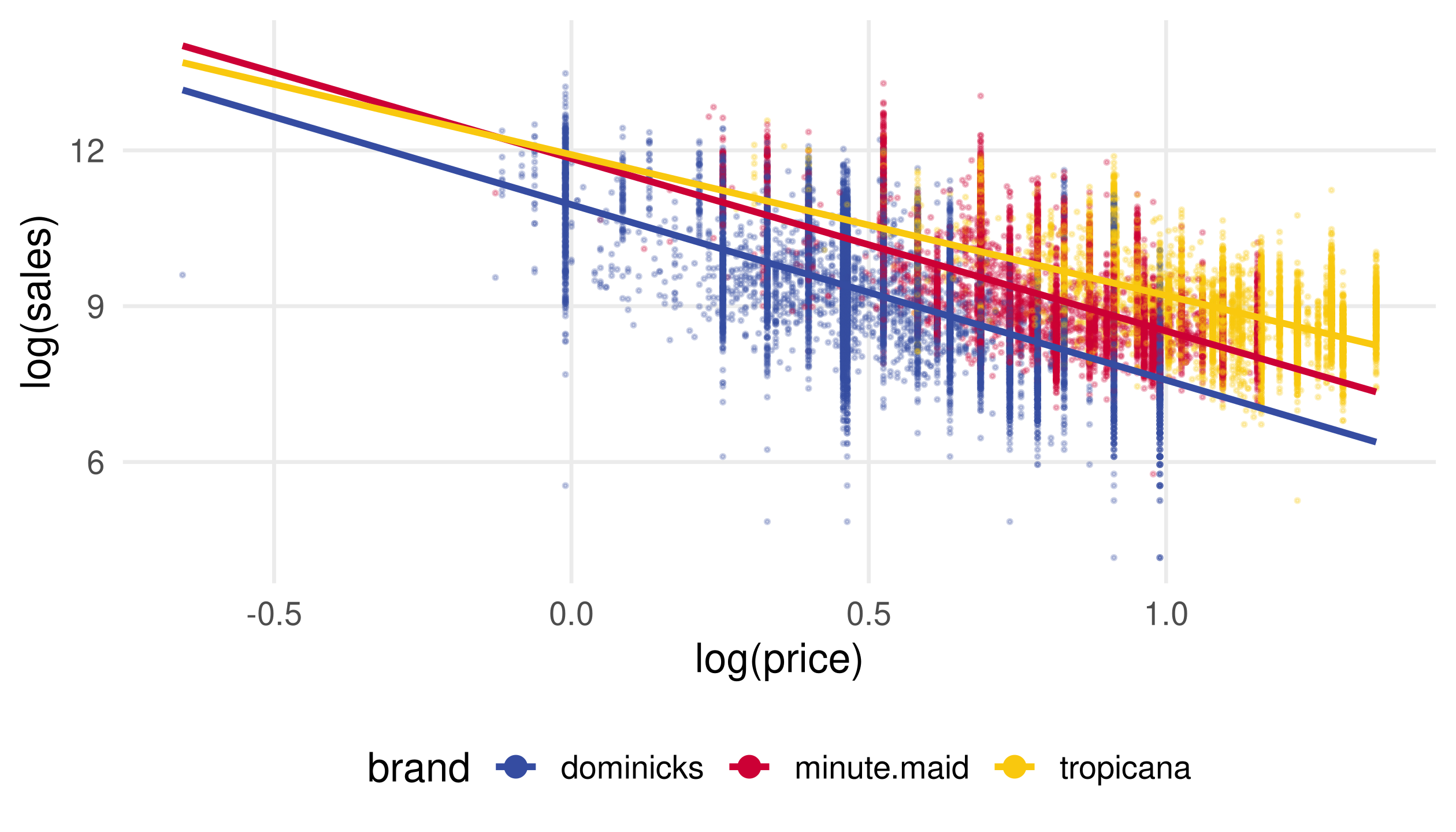
Tropicana buyers are the least price sensitive: a 1% price increase goes with about 2.7% lower sales, against 3.4% for Dominick’s.

b[["log(price)"]] extracts one number by name; [[ drops the old name so that c() can attach a clean one.

Tropicana’s demand curve is flatter

Scatterplot of log sales against log price by brand with three fitted lines from the interaction model. The Tropicana line is visibly flatter than the Dominick's and Minute Maid lines.

Same recipe as before: predict from the interaction model on the grid, then draw the lines.

Add advertising to the model

feat records whether the brand was featured in the store that week. Interact everything:

OLS_full_interactions_model <- glm(log(sales) ~ log(price) * brand * feat, data = oj)
round(coef(summary(OLS_full_interactions_model)), 3)
##                                  Estimate Std. Error t value Pr(>|t|)
## (Intercept)                        10.407      0.023 445.668    0.000
## log(price)                         -2.774      0.039 -71.445    0.000
## brandminute.maid                    0.047      0.047   1.012    0.311
## brandtropicana                      0.708      0.051  13.937    0.000
## feat                                1.094      0.038  28.721    0.000
## log(price):brandminute.maid         0.783      0.061  12.750    0.000
## log(price):brandtropicana           0.736      0.057  12.946    0.000
## log(price):feat                    -0.471      0.074  -6.351    0.000
## brandminute.maid:feat               1.173      0.082  14.312    0.000
## brandtropicana:feat                 0.785      0.099   7.952    0.000
## log(price):brandminute.maid:feat   -1.109      0.122  -9.074    0.000
## log(price):brandtropicana:feat     -0.986      0.124  -7.946    0.000

log(price) * brand * feat includes all main effects, all pairwise products, and the three-way product. The 12 coefficients give an intercept and a slope for each of the six brand-by-promotion cells.

Elasticities with and without promotion

Each cell’s slope is the baseline slope plus every interaction that is switched on:

b <- coef(OLS_full_interactions_model)
lp <- "log(price)"
el <- rbind(
  no_ad = c(b[lp], b[lp] + b["log(price):brandminute.maid"],
            b[lp] + b["log(price):brandtropicana"]),
  ad    = c(b[lp] + b["log(price):feat"],
            b[lp] + b["log(price):brandminute.maid"] + b["log(price):feat"] +
              b["log(price):brandminute.maid:feat"],
            b[lp] + b["log(price):brandtropicana"] + b["log(price):feat"] +
              b["log(price):brandtropicana:feat"]))
colnames(el) <- levels(oj$brand)
round(el, 2)
##       dominicks minute.maid tropicana
## no_ad     -2.77       -1.99     -2.04
## ad        -3.24       -3.57     -3.50

Promotion makes every brand’s demand more elastic, and the ranking across brands changes.

Why does promotion raise elasticity?

More elastic with ads. A feature ad reaches shoppers beyond the brand loyalists, and these marginal customers respond more to price. Promotions also tend to coincide with price cuts, and stocking up amplifies the response.

The ranking changed. Without feat, Minute Maid looked as price sensitive as Dominick’s (-3.32 against -3.38) while Tropicana stood apart (-2.71). With feat, Minute Maid and Tropicana look alike within each promotion state.

Something correlated with brand and with sales was missing from the earlier model.

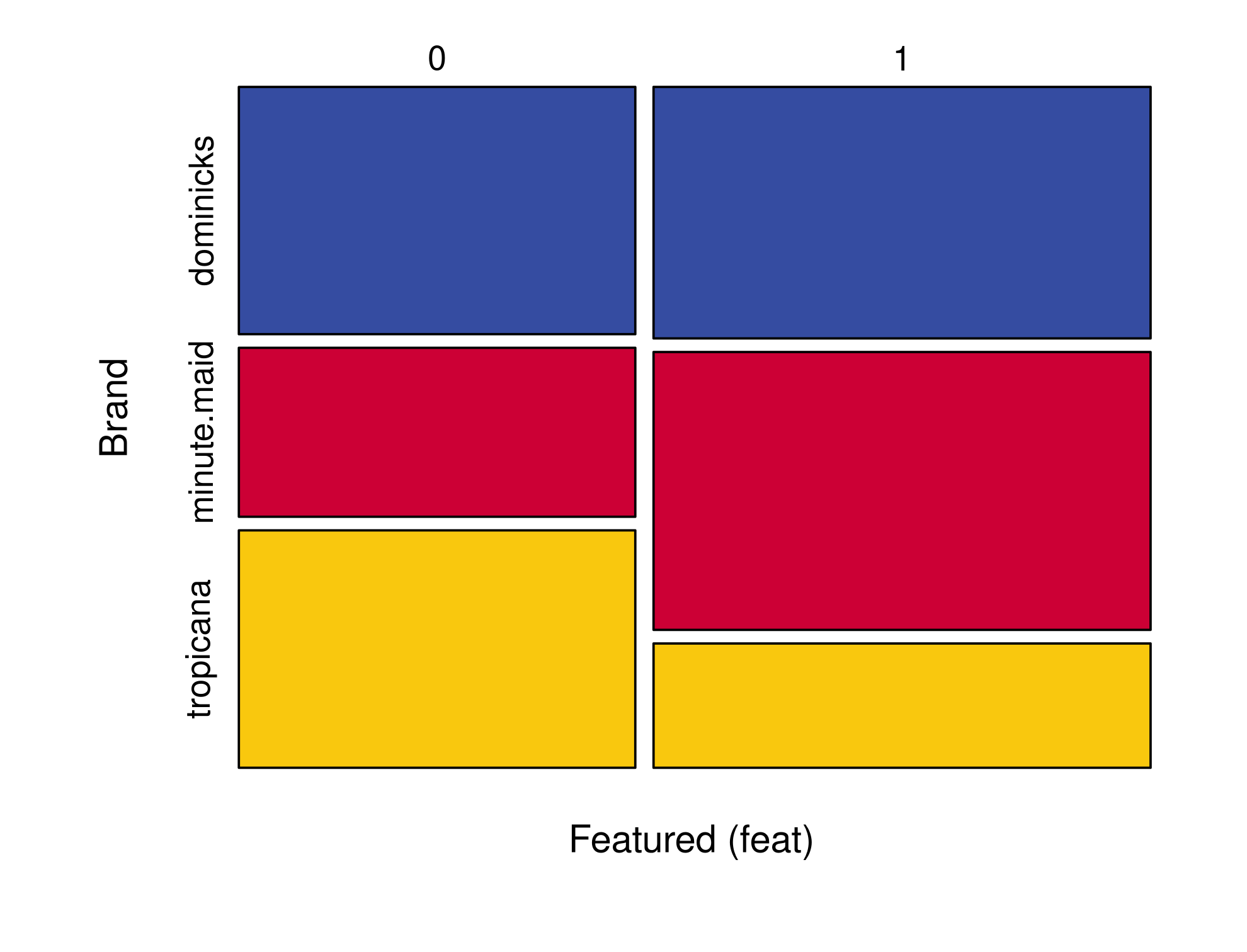
Minute Maid sells more through promotions

sales_by_ads <- tapply(oj$sales,
                       oj[, c("feat", "brand")], sum)
round(prop.table(sales_by_ads, margin = 2), 2)
##     brand
## feat dominicks minute.maid tropicana
##    0      0.44        0.33       0.6
##    1      0.56        0.67       0.4

Two-thirds of Minute Maid’s units are sold in featured weeks, against 40% of Tropicana’s.

Mosaic plot of total sales by advertising status and brand. Featured weeks account for a much larger share of Minute Maid sales than of Tropicana sales.

Omitting promotion biased the brand elasticities

Minute Maid’s sales came disproportionately from featured weeks, which combine low prices with high volumes.

Without feat, the price coefficient for Minute Maid absorbs the promotion effect, so Minute Maid looks as price sensitive as the store brand.

Omitted-variable bias. A left-out variable that is correlated with an included regressor and affects the outcome shifts the regressor’s coefficient. The coefficient then describes a different comparison from the intended one.

We return to this logic with the housing data, where it appears in a two-regressor model.

Predict for new observations

Given X_{n+1}, the prediction is X_{n+1}'\hat\beta. predict() builds the row of the model matrix for us:

new_dat <- data.frame(price = c(3, 3.5, 2),
                      brand = c("tropicana", "minute.maid", "dominicks"),
                      feat  = c(0, 0, 1))
exp(predict(OLS_model, newdata = new_dat))   # predicted units, not log units
##        1        2        3 
## 7409.805 2361.282 5728.715
  • new_dat must contain every variable in the model’s formula, with brand labels that match the factor levels.
  • OLS_model does not use feat, so that column is ignored here; the full model would use it.
  • The model predicts log sales, so we exponentiate to get units sold.

Checkpoint: read the orange-juice models

  1. In OLS_model, the Tropicana coefficient is 1.53. Is Tropicana’s sales advantage 153%?
  2. In the interaction model, which coefficient answers “do Tropicana buyers respond to price differently from Dominick’s buyers”?
  3. Why did adding feat change the Minute Maid elasticity so much more than the Tropicana elasticity?
  4. Which model should you use to predict next week’s sales during a promotion?

One-bedroom condos in Los Angeles


Confounding, multicollinearity, and interactions with few observations

133 listings from October 2023

redfin <- read.csv("./data/redfinLA3.csv")
dim(redfin)
## [1] 133  27
redfin %>% count(LOCATION)
##                  LOCATION  n
## 1     C42 - Downtown L.A. 35
## 2           Downtown L.A. 80
## 3 Westwood - Century City 18

One-bedroom condos for sale, downloaded from Redfin and filtered to the three locations with the most listings.

Variable Meaning
PRICE Listing price ($)
SQUARE_FEET Interior size
BATHS Bathrooms: 1, 1.5, 2, or 2.5
LOCATION Neighbourhood label from the listing service

Price against size and bathrooms

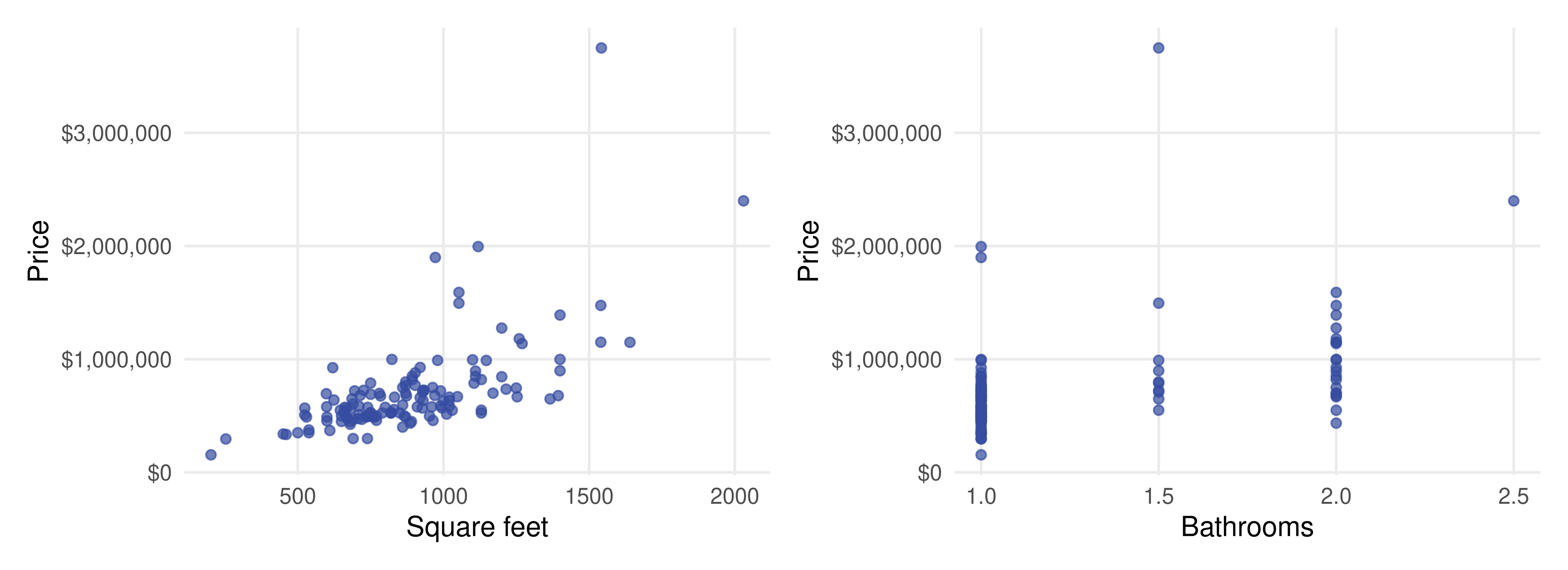
Two scatterplots. Left: listing price rises with square footage, roughly linearly, with a few very expensive outliers. Right: price against number of bathrooms, which takes only four values, with wide vertical spread at each value.

Price rises with size in a roughly linear way, with substantial spread. Bathrooms take four values, so the right panel is really four conditional distributions.

Start with bathrooms alone

fit_baths <- lm(PRICE ~ BATHS, data = redfin)
printCoefmat(coef(summary(fit_baths)))
##             Estimate Std. Error t value  Pr(>|t|)    
## (Intercept)   106782     105909  1.0082    0.3152    
## BATHS         500430      83542  5.9902 1.899e-08 ***
## ---
## Signif. codes:  0 '***' 0.001 '**' 0.01 '*' 0.05 '.' 0.1 ' ' 1

Each additional bathroom goes with about $500,000 more in listing price.

Is that the value of a bathroom? Condos with more bathrooms are also larger.

Add square footage

fit_size <- lm(PRICE ~ BATHS + SQUARE_FEET, data = redfin)
printCoefmat(coef(summary(fit_size)))
##               Estimate Std. Error t value  Pr(>|t|)    
## (Intercept) -216002.95  102181.89 -2.1139   0.03643 *  
## BATHS        112732.45   91015.62  1.2386   0.21772    
## SQUARE_FEET     892.04     128.98  6.9160 1.891e-10 ***
## ---
## Signif. codes:  0 '***' 0.001 '**' 0.01 '*' 0.05 '.' 0.1 ' ' 1

The bathrooms coefficient falls from about $500,000 to about $113,000 and is no longer statistically distinguishable from zero. Its standard error rises.

cor(redfin$BATHS, redfin$SQUARE_FEET)
## [1] 0.6159194

Bathrooms and size are strongly correlated. The first model credited bathrooms with the effect of size.

Two consequences of correlated regressors

Omitted-variable bias, a bias problem. Size affects price and is correlated with bathrooms. Leaving size out makes the bathrooms coefficient absorb part of the size effect.

Multicollinearity, a precision problem. With both included, the data contain little independent variation in bathrooms at a given size, so the bathrooms coefficient is estimated less precisely.

Model BATHS estimate BATHS std. error
PRICE ~ BATHS 500,430 83,542
PRICE ~ BATHS + SQUARE_FEET 112,732 91,016

A coefficient is defined relative to the other regressors in the model. Changing the model changes the question it answers.

Signs can flip: Simpson’s paradox

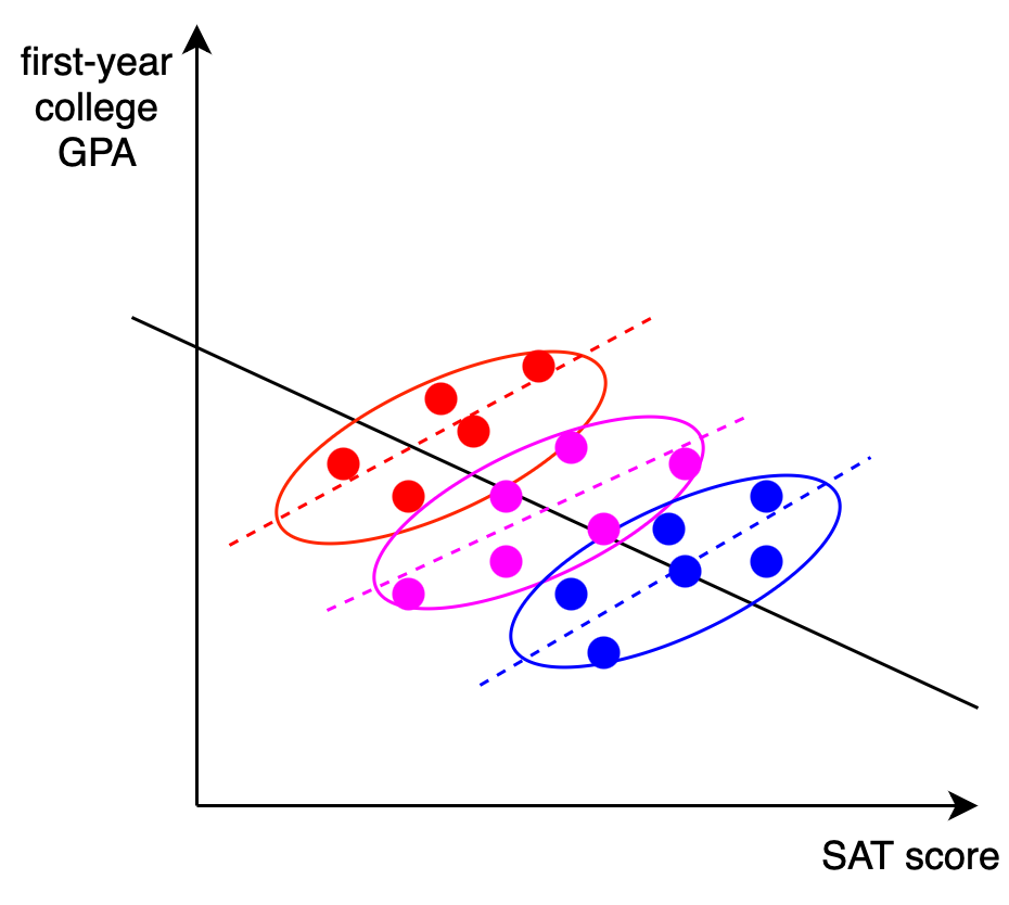
Regress first-year college GPA on SAT score for one high-school graduating class.

  • Across the whole class, the relationship is negative.
  • Within each college the students attend, it is positive.

Students with higher scores enter more selective colleges, where grades are harder to earn. College is a confounder that reverses the sign.

Conditioning on a third variable can change a coefficient’s size, its precision, or its sign.

Stylized scatterplot of first-year college GPA against SAT score. Three coloured clusters of students, one per college, each slope upward, while the black line fitted to all students slopes downward.

Location as a categorical regressor

fit_location <- lm(PRICE ~ LOCATION, data = redfin)
printCoefmat(coef(summary(fit_location)))
##                                 Estimate Std. Error t value  Pr(>|t|)    
## (Intercept)                       656834      69749  9.4171 2.259e-16 ***
## LOCATIONDowntown L.A.              22927      83626  0.2742   0.78439    
## LOCATIONWestwood - Century City   295994     119685  2.4731   0.01468 *  
## ---
## Signif. codes:  0 '***' 0.001 '**' 0.01 '*' 0.05 '.' 0.1 ' ' 1

LOCATION is a character column; lm() converts it to a factor and creates two indicators. The baseline is the first level alphabetically, “C42 - Downtown L.A.”.

Westwood listings are about $296,000 more expensive on average than the baseline; the two Downtown labels are indistinguishable.

Size and location: parallel slopes

fit_location_size <- lm(PRICE ~ SQUARE_FEET + LOCATION, data = redfin)
printCoefmat(coef(summary(fit_location_size)))
##                                    Estimate  Std. Error t value  Pr(>|t|)    
## (Intercept)                     -215184.799   92730.256 -2.3205 0.0218809 *  
## SQUARE_FEET                        1066.559      95.563 11.1608 < 2.2e-16 ***
## LOCATIONDowntown L.A.            -99820.232   60880.033 -1.6396 0.1035203    
## LOCATIONWestwood - Century City  299833.249   85698.107  3.4987 0.0006422 ***
## ---
## Signif. codes:  0 '***' 0.001 '**' 0.01 '*' 0.05 '.' 0.1 ' ' 1

Every location shares the same price per square foot, about $1,070. Westwood commands roughly $300,000 more at the same size.

Is one price per square foot plausible across neighbourhoods?

Let price per square foot vary by location

fit_interaction <- lm(PRICE ~ SQUARE_FEET * LOCATION, data = redfin)
printCoefmat(coef(summary(fit_interaction)))
##                                                Estimate  Std. Error t value  Pr(>|t|)    
## (Intercept)                                  -78035.534  179343.778 -0.4351  0.664216    
## SQUARE_FEET                                     898.813     212.439  4.2309 4.421e-05 ***
## LOCATIONDowntown L.A.                        -16696.031  206152.434 -0.0810  0.935578    
## LOCATIONWestwood - Century City             -747908.233  255326.342 -2.9292  0.004029 ** 
## SQUARE_FEET:LOCATIONDowntown L.A.               -68.425     236.657 -0.2891  0.772954    
## SQUARE_FEET:LOCATIONWestwood - Century City    1286.410     298.527  4.3092 3.254e-05 ***
## ---
## Signif. codes:  0 '***' 0.001 '**' 0.01 '*' 0.05 '.' 0.1 ' ' 1

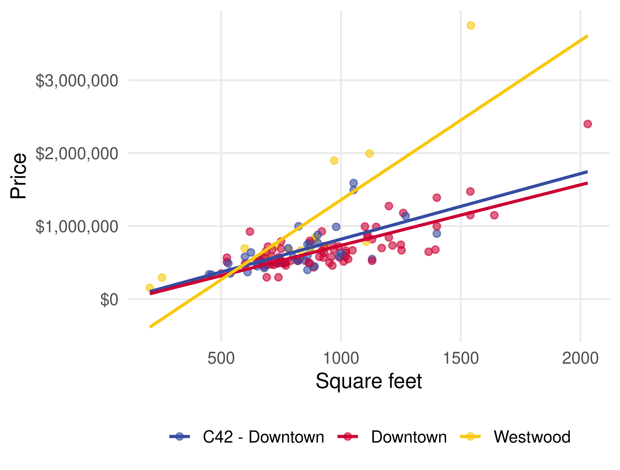
Westwood’s price per square foot is about $899 + $1,286 = $2,185. The two Downtown labels stay near $900 and $830.

Different lines for different neighbourhoods

grid_la <- expand.grid(
  SQUARE_FEET = seq(min(redfin$SQUARE_FEET),
                    max(redfin$SQUARE_FEET),
                    length.out = 100),
  LOCATION = unique(redfin$LOCATION))
grid_la$PRICE <- predict(fit_interaction,
                         newdata = grid_la)

grid_la has 300 rows: 100 sizes for each location. predict() applies the location-specific intercept and slope to each row.

The plot uses the same recipe as the orange-juice slides: points from redfin, lines from grid_la.

Scatterplot of condo price against square feet coloured by location, with a fitted line per location. The Westwood line is much steeper than the two Downtown lines, which are nearly parallel.

The Westwood line rests on 18 listings. Interactions double the parameters spent on location.

Checkpoint: which model prices a condo?

A client asks what a 900 square-foot, one-bathroom Westwood condo should list for.

  1. Which of the fitted models would you use, and what does it predict?
  2. In the interaction model, the Westwood indicator is about -748{,}000 dollars. Is Westwood cheaper?
  3. What would you check before trusting the Westwood slope?

Regression estimates conditional means

Define the target. \mathbf{E}[Y \mid X] is the prediction. OLS approximates it with a line and remains the best linear predictor when the truth is curved.

Build the design. Indicators encode categories, logs turn slopes into elasticities, and interactions let slopes differ across groups.

Read coefficients conditionally. A coefficient is a comparison holding the other regressors fixed. Adding or removing a regressor changes the question.

Keep correlation and causation apart. Omitted promotions and omitted size both shifted coefficients. A regression describes an association in the data at hand.

Reading and data sources

Additional details


Robust standard errors, alternative codings, and the OLS formula

Heteroskedasticity: error variance that moves with X

summary() computes standard errors that assume homoskedasticity:

\text{Var}(\varepsilon_i \mid X_i) = \sigma^2 \quad \text{for all } i.

Under heteroskedasticity, the variance depends on the covariates:

\text{Var}(\varepsilon_i \mid X_i) = \sigma^2(X_i).

Common in economic data: price dispersion grows with home value, earnings dispersion grows with education, and revenue dispersion grows with firm size.

A simulated example

set.seed(123)
n <- 500
X <- sample(0:3, n, replace = TRUE)
eps <- rnorm(n, mean = 0, sd = sqrt(0.5 + X))
Y <- 0.5 + 3 * X + eps
het <- data.frame(X, Y)

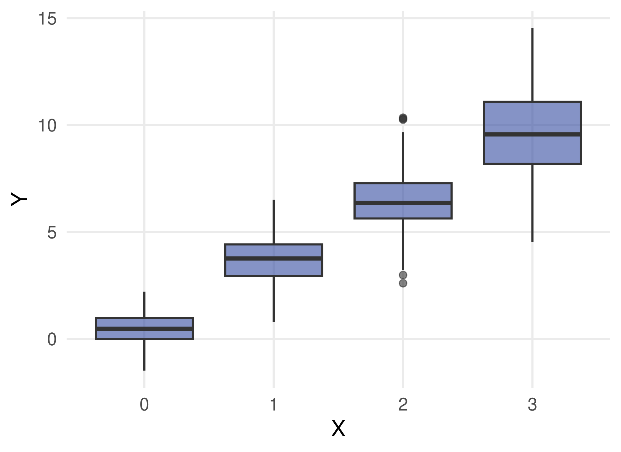
The error standard deviation is \sqrt{0.5 + X}, so the spread of Y around the line fans out as X grows.

Boxplots of simulated Y at X equal to 0, 1, 2 and 3. The medians rise linearly and the boxes and whiskers widen as X increases.

Consequences of heteroskedasticity

Quantity Under heteroskedasticity
OLS point estimates Still unbiased and consistent
summary() standard errors Wrong
t-tests and confidence intervals Unreliable

Heteroskedasticity does not affect the validity of \hat\beta. It affects inference about \beta.

Use heteroskedasticity-robust standard errors whenever heteroskedasticity is plausible. In economic data, that is most of the time.

Robust standard errors in R

The sandwich package supplies the robust covariance matrix; coeftest() from lmtest reports the table.

library(sandwich); library(lmtest)
fit_het <- lm(Y ~ X, data = het)
coeftest(fit_het, vcov = sandwich)
## 
## t test of coefficients:
## 
##             Estimate Std. Error t value  Pr(>|t|)    
## (Intercept) 0.535809   0.068879   7.779 4.243e-14 ***
## X           2.997983   0.060590  49.480 < 2.2e-16 ***
## ---
## Signif. codes:  0 '***' 0.001 '**' 0.01 '*' 0.05 '.' 0.1 ' ' 1
cbind(conventional = coef(summary(fit_het))[, "Std. Error"],
      robust = sqrt(diag(sandwich(fit_het))))
##             conventional     robust
## (Intercept)   0.09963804 0.06887871
## X             0.05606852 0.06058990

The estimates are unchanged. Robust standard errors can be larger or smaller than the conventional ones.

Alternative codings of a factor

Dropping the intercept gives one indicator per brand; relevel() changes the baseline. Both are reparameterizations with identical fitted values.

coef(glm(log(sales) ~ log(price) + brand - 1, data = oj))
##       log(price)   branddominicks brandminute.maid   brandtropicana 
##        -3.138691        10.828822        11.698996        12.358764
oj_trop <- mutate(oj, brand = relevel(brand, ref = "tropicana"))
coef(glm(log(sales) ~ log(price) + brand, data = oj_trop))
##      (Intercept)       log(price)   branddominicks brandminute.maid 
##       12.3587643       -3.1386914       -1.5299428       -0.6597681

Without an intercept, each brand coefficient is that brand’s own intercept. With Tropicana as the baseline, the other two brands’ coefficients become negative shifts.

Where the OLS formula comes from

Differentiate the sum of squared residuals with respect to b and set the result to zero:

\frac{\partial}{\partial b}\sum_{i=1}^n (Y_i - X_i'b)^2 = -2\sum_{i=1}^n X_i\,(Y_i - X_i'b) = 0.

Rearranging gives the normal equations and their solution:

\sum_{i=1}^n X_iX_i'\,\hat\beta = \sum_{i=1}^n X_iY_i \quad\Longrightarrow\quad \hat\beta = \left(\sum_{i=1}^n X_iX_i'\right)^{-1}\sum_{i=1}^n X_iY_i.

The inverse exists when no regressor is a linear combination of the others. That is why a factor with an intercept needs one fewer indicator than levels.

Check the formula by hand

model.matrix() returns the n \times d matrix whose rows are the X_i'; crossprod() computes the sums.
Xmat <- model.matrix(OLS_model)
y <- log(oj$sales)
by_hand <- solve(crossprod(Xmat), crossprod(Xmat, y))   # (X'X)^{-1} X'y
cbind(by_hand = drop(by_hand), lm = coef(OLS_model))
##                     by_hand         lm
## (Intercept)      10.8288216 10.8288216
## log(price)       -3.1386914 -3.1386914
## brandminute.maid  0.8701747  0.8701747
## brandtropicana    1.5299428  1.5299428

lm() uses a numerically more stable QR decomposition rather than this inverse, but the answer is the same.

lm() versus glm()

lm() glm() with the Gaussian family
Estimates OLS The same numbers
Fit statistics in summary() R^2, F-test, residual standard error Deviance, AIC, dispersion
Extends to Weighted least squares Logit, Poisson, and other families
all.equal(coef(lm(log(sales) ~ log(price) + brand, data = oj)), coef(OLS_model))
## [1] TRUE

For OLS, choose whichever output you prefer. Next lecture, glm(..., family = binomial) fits a logistic regression with the same formula.

Install the required packages

Run once in your R environment if needed:

install.packages(c("tidyverse", "patchwork", "sandwich", "lmtest"))

The three datasets are in lectures/data/ and the Simpson’s paradox figure in lectures/images/, so the deck renders without network access.

Return to the research question

What is the outcome, what is being held fixed, and what comparison does each coefficient describe?

Those questions decide which conclusions a regression can support.

Return to the main takeaway