policy_text <- tibble(
  document = 1:3,
  text = c(
    "The committee monitors inflation and employment.",
    "Inflation risks remain, but employment is growing.",
    "The committee is not raising interest rates."
  )
)
tokens <- policy_text %>% unnest_tokens(word, text)ECON 4370 / 6370 Computing for Economics
Lecture 8: Text as Data
Zhan Gao
14 September 2026
What can language tell us?
| Text | A measurable question |
|---|---|
| Congressional speech | How does phrase use vary with constituency politics? |
| Restaurant reviews | Which recurring themes appear together? |
| Monetary-policy statements | How does emphasis change across documents? |
Text becomes data only after we define a document, a vocabulary, and a measurement rule.
Today’s route
- Represent text: turn documents into token counts.
- Relate text to an outcome: examine congressional speech.
- Discover recurring themes: build and interpret topic mixtures.
- Read the evidence: analyze restaurant reviews.
Additional code and model details follow the main lesson.
Packages and data
Run the examples from the lectures/ directory.
| Tool / data | Role |
|---|---|
tidytext, SnowballC |
Tokenization and stemming |
congress109 in textir |
Congressional phrase counts and member attributes |
we8there in textir |
Restaurant-review phrase counts and ratings |
slam, maptpx |
Sparse count storage and topic estimation |
Both research datasets are bundled with textir, as in the notes.
Represent text
Choose what to keep before counting it
The document defines the observation
A corpus is a collection of documents. A token is a unit of text we count.
| Choice | Example |
|---|---|
| Document | One review, one speech, or one speaker’s annual speeches |
| Token | A word, a two-word phrase, or a three-word phrase |
| Vocabulary | The set of retained tokens shared across documents |
Combining all of a speaker’s speeches changes the question: we study the speaker’s aggregate language, not variation across speeches.
Bag of words discards order
These two illustrative sentences have the same word counts:
Workers support firms.
Firms support workers.
| Document | firms | support | workers |
|---|---|---|---|
| Sentence 1 | 1 | 1 | 1 |
| Sentence 2 | 1 | 1 | 1 |
The representation keeps vocabulary and repetition; it loses who supports whom.
A matrix makes the representation explicit
Let X have n document rows and d token columns:
X_{ij}=\text{number of times token }j\text{ appears in document }i.
| Document | bank | loan | rate | m_i=\sum_j X_{ij} |
|---|---|---|---|---|
| A: “bank loan loan” | 1 | 2 | 0 | 3 |
| B: “bank rate” | 1 | 0 | 1 | 2 |
After pruning, m_i counts retained tokens. It may differ from the original document’s word count.
Tokenize a small policy example
The following are illustrative sentences, not quotations from an FOMC release.
By default, unnest_tokens() lowercases words and returns one token per row.
Count within each document
## # A tibble: 6 × 3
##   document word           n
##      <int> <chr>      <int>
## 1        1 committee      1
## 2        1 employment     1
## 3        1 inflation      1
## 4        2 employment     1
## 5        2 inflation      1
## 6        3 committee      1
The document ID stays attached to each token. An absent document–word pair represents a zero count.
Preprocessing changes the evidence
| Operation | What it does | What can be lost |
|---|---|---|
| Lowercase | Treat Bank and bank alike |
Proper-name distinctions |
| Remove stopwords | Drop a chosen list of common words | Negation: “not raising” |
| Stem | Merge some related word forms | Grammatical distinctions |
| Drop rare tokens | Reduce vocabulary size | Unusual but informative phrases |
Choose preprocessing for the question. More pruning does not automatically mean better measurement.
Stopwords require a judgment call
## # A tibble: 3 × 2
##   document word
##      <int> <chr>
## 1        3 committee
## 2        3 raising
## 3        3 rates
The original sentence says “not raising interest rates.” The default list removes both “not” and “interest.”
For a question about policy direction, preserve negation or encode meaningful phrases.
Stems need not be dictionary words
## # A tibble: 5 × 2
##   word      stem
##   <chr>     <chr>
## 1 write     write
## 2 writes    write
## 3 writing   write
## 4 written   written
## 5 inflation inflat
Stemming uses language-specific rules. It does not recover every grammatical root: “written” remains distinct here.
Bigrams retain local order
## # A tibble: 6 × 2
##   document bigram
##      <int> <chr>
## 1        3 the committee
## 2        3 committee is
## 3        3 is not
## 4        3 not raising
## 5        3 raising interest
## 6        3 interest rates
A bigram contains two adjacent words; a trigram contains three. Longer phrases expand the vocabulary and are usually sparser.
Filtering first can invent adjacency
Start with the phrase “quality of service.”
| Order of operations | Result |
|---|---|
| Form bigrams first | quality of, of service |
Then remove any bigram containing of |
No surviving bigram |
Remove of first, then form bigrams |
quality service |
The last row creates a pair that was never adjacent in the original text.
If original adjacency matters, form phrases before removing stopwords or stemming their components.
Rare means rare across documents
The document frequency of token j is
\mathrm{df}_j=\sum_{i=1}^{n}\mathbf{1}\{X_{ij}>0\}.
A token repeated 100 times in one document still has document frequency 1.
The cutoff above is a recipe for a larger corpus. Check sensitivity to the cutoff.
Build a sparse document–term matrix
## 3 x 3 sparse Matrix of class "dgCMatrix"
##   committee employment inflation
## 1         1          1         1
## 2         .          1         1
## 3         1          .         .
Rows are documents; columns are tokens. Dots in the sparse printout are zeros.
Checkpoint: what did we measure?
Consider two reviews:
“Good service.”
“Not good service.”
- How does a word-count representation distinguish them?
- What happens if “not” is removed?
- Which bigram preserves the difference?
- Does stemming solve the negation problem?
Relate text to an outcome
Congressional language and constituency politics
One row is one speaker’s year
The congress109 example aggregates each legislator’s speeches from the 2005 Congressional Record.
## [1] 529 1000There are 529 speakers × 1,000 phrases: 500 bigrams and 500 trigrams, already processed.
A few entries reveal the representation
## 2 x 4 sparse Matrix of class "dgCMatrix"
##              stem.cel natural.ga hurricane.katrina trade.agreement
## Barack Obama        .          1                20               7
## John Boehner        .          .                14               .
stem.cel and natural.ga illustrate the supplied stemming. Dots between words join a phrase; they are not sentence punctuation.
Each cell is a count across that speaker’s 2005 speeches.
Define the outcome before fitting
| Field | Meaning |
|---|---|
party, state, chamber |
Speaker attributes; chamber is House or Senate |
repshare |
Bush’s share of the two-party presidential vote in 2004 |
cs1, cs2 |
Ideological common scores derived from roll-call voting |
For repshare, the constituency is a House district or, for senators, a state.
repshare = 0.79 means 79% of the constituency’s two-party presidential vote went to Bush. It is not the speaker’s party-line voting rate.
Find phrases associated with vote share
- Positive covariance: higher counts tend to occur in constituencies with higher Bush vote shares.
- Negative covariance: higher counts tend to occur in constituencies with lower Bush vote shares.
- Magnitudes depend on phrase frequency and how much each speaker talks.
This is a marginal association. It is not a causal effect or a classification of every speaker.
Phrase associations have a direction
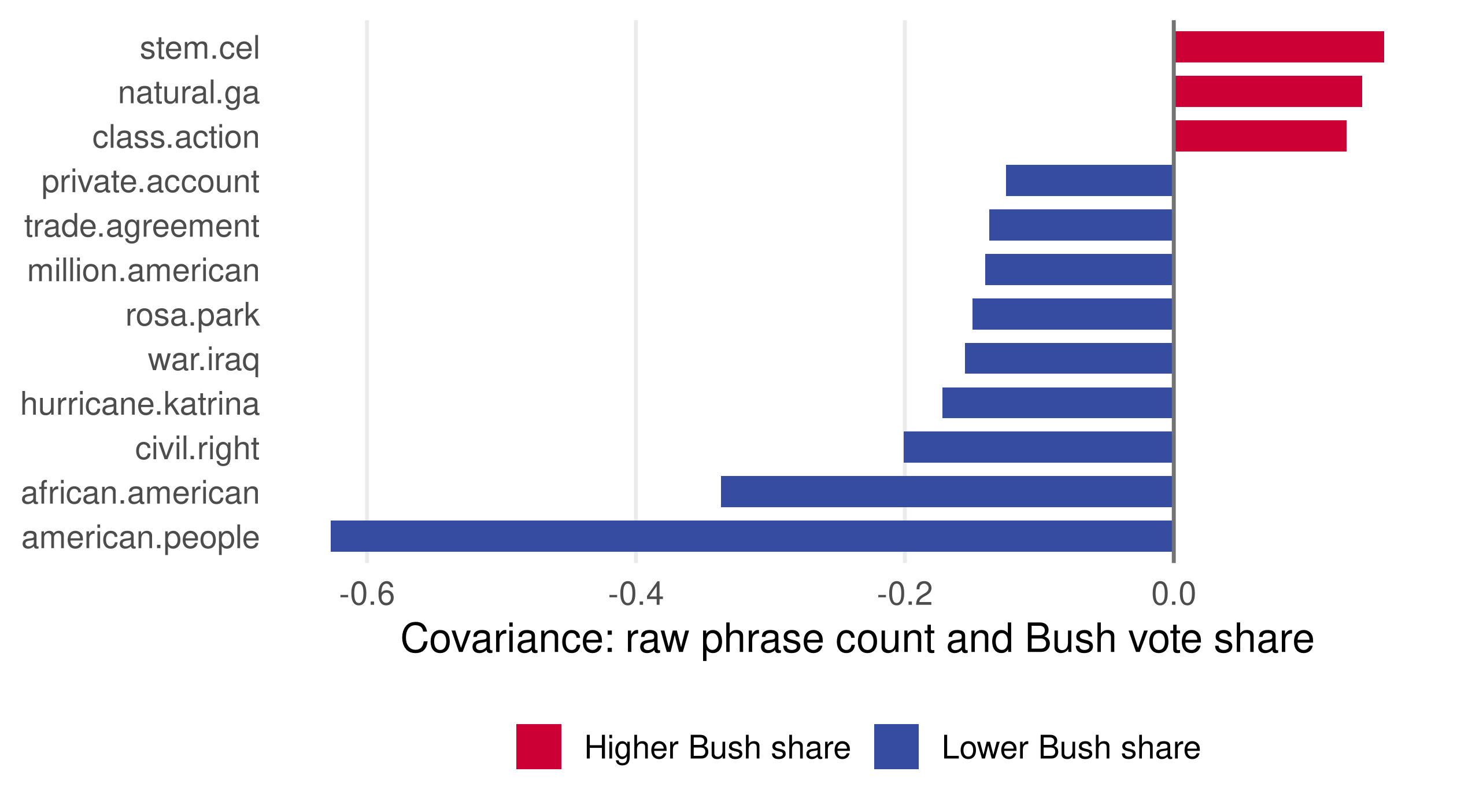
The scale shows both sign and magnitude; frequent phrases can dominate this ranking.
Counts, shares, and indicators differ
Let m_i=\sum_{j=1}^{1000}X_{ij}, the count across the full retained vocabulary.
| Feature | Definition | What it emphasizes |
|---|---|---|
| Raw count | X_{ij} | Repetition and speaking volume |
| Phrase share | X_{ij}/m_i | Relative use within retained phrases |
| Indicator | \mathbf{1}\{X_{ij}>0\} | Whether a phrase appears at all |
Compute m_i before selecting a few predictors. A total over only the selected phrases defines a different denominator.
Fit a small descriptive regression
top_words <- names(sort(abs(assocs), decreasing = TRUE))[1:20]
x_count <- as.matrix(counts[, top_words])
total <- Matrix::rowSums(counts)
stopifnot(all(total > 0))
x_share <- sweep(x_count, 1, total, "/")
x_present <- 1L * (x_count > 0)

fit_count <- lm(y ~ ., data = data.frame(x_count))
fit_share <- lm(y ~ ., data = data.frame(x_share))
fit_present <- lm(y ~ ., data = data.frame(x_present))
The same 20 phrases enter each specification. Their ranking was chosen using this sample’s outcome.
Read coefficients conditionally
For the raw-count model,
\widehat y_i=\widehat\beta_0+\sum_{j\in S}\widehat\beta_j X_{ij}, \qquad |S|=20.
- A positive coefficient means a higher fitted Bush vote share when that count rises, holding the other included counts fixed.
- This sign can differ from the marginal covariance because phrases co-occur.
- Coefficients have different units across count, share, and indicator models.
The outcome describes constituents. A coefficient is not an effect of saying a phrase on election results.
More regressors can improve training fit
x_all <- cbind(x_count, x_share, x_present)
colnames(x_all) <- make.unique(colnames(x_all))
fit_all <- lm(y ~ ., data = data.frame(x_all))
fits <- list(Counts = fit_count, Shares = fit_share,
             Indicators = fit_present, Combined = fit_all)
tibble(Model = names(fits),
       `Training R-squared` = map_dbl(fits, ~ summary(.x)$r.squared)) %>%
knitr::kable(digits = 3)| Model | Training R-squared |
|---|---|
| Counts | 0.217 |
| Shares | 0.292 |
| Indicators | 0.313 |
| Combined | 0.424 |
Adding predictors cannot reduce ordinary training R^2 for nested OLS models on the same observations.
Training fit is not prediction performance
The comparison answers: How well do these specifications fit the observed sample?
It does not establish which will predict new speakers best.
- We selected the top 20 phrases using the same outcome we then fitted.
- The supplied 1,000-phrase vocabulary was already selected using party labels.
- Some speakers share a constituency outcome; a random row split may place related observations on both sides.
For new prediction work, define the split first and learn the vocabulary and feature choices within training data.
Political speech is a measurement problem
Our example: relate 2005 phrase use to constituency vote share.
Media slant: compare newspaper language with phrases associated with congressional parties (Gentzkow and Shapiro, 2010).
Historical partisanship: measure how well speech distinguishes parties, accounting for bias in high-dimensional comparisons (Gentzkow, Shapiro and Taddy, 2019).
These are related questions with different units, outcomes, and estimands.
Checkpoint: what would you conclude?
A combined count/share/indicator model has the largest training R^2.
- Does that make it the best predictor for a future Congress?
- Would selecting phrases on the full sample before splitting solve the problem?
- What does a positive coefficient actually describe here?
Separate three tasks: defining a construct, describing an association, and evaluating prediction.
Discover recurring themes
Describe language even when documents have no outcome labels
A document can mix several topics
A restaurant review might discuss food, service, and price in the same paragraph.
A topic model represents this overlap with two sets of probabilities:
| Quantity | Question |
|---|---|
| Topic–word probability \theta_{kj} | Within topic k, how likely is token j? |
| Document–topic weight \omega_{ik} | For document i, how much weight goes to topic k? |
Topic names come from our interpretation of the fitted probabilities. They are not supplied to the model.
The two probability constraints
A topic allocates probability across the vocabulary:
\theta_{kj}\geq0,\qquad \sum_{j=1}^{d}\theta_{kj}=1 \quad\text{for each topic }k.
A document allocates weight across topics:
\omega_{ik}\geq0,\qquad \sum_{k=1}^{K}\omega_{ik}=1 \quad\text{for each document }i.
Knowing a document’s topic weights does not tell us the order of its words.
Generate one token at a time
Imagine a document with m_i retained tokens.
- Draw a topic k using the document’s weights \omega_i.
- Draw a token j using that topic’s probabilities \theta_k.
- Repeat m_i times, then count the tokens.
The resulting probability of token j is
p_{ij}=\sum_{k=1}^{K}\omega_{ik}\theta_{kj}.
This is a model for the counts, not a literal claim about how people write.
A small mixture you can calculate
Consider an illustrative vocabulary and two topics:
| Topic | food | service | price |
|---|---|---|---|
| Topic 1 | 0.60 | 0.30 | 0.10 |
| Topic 2 | 0.10 | 0.30 | 0.60 |
A document with weights (0.75,\ 0.25) has token probabilities
0.75(0.60,0.30,0.10)+0.25(0.10,0.30,0.60) =(0.475,0.300,0.225).
For 100 retained tokens, expected counts are (47.5,30,22.5); observed counts are random integers.
The count vector is multinomial
Conditional on the document’s length and topic weights,
X_i\mid m_i,\omega_i,\Theta\sim \operatorname{Multinomial}\!\left(m_i,\sum_{k=1}^{K}\omega_{ik}\theta_k\right).
Consequently,
\mathbb{E}\!\left[\frac{X_i}{m_i}\mid\omega_i,\Theta\right] =\sum_{k=1}^{K}\omega_{ik}\theta_k.
Latent Dirichlet allocation (LDA) places a Dirichlet distribution on the document-topic weights: a distribution over probability vectors.
Topic mixtures and PCA answer differently
| Aspect | PCA / linear factors | Topic model |
|---|---|---|
| Representation | Weighted linear combination | Mixture of token probabilities |
| Scores / weights | Can be negative | Nonnegative and sum to one |
| Loadings | Depend on scaling and centering | Each topic is a probability vector |
| Interpretation | Latent dimensions | Recurring token distributions |
Both reduce dimension, and both require interpretation. PCA can be applied to text features; LDA explicitly models token counts.
Estimation needs a model and an algorithm
We observe the count matrix X. We estimate both the topic distributions and the document weights.
maptpx fits a maximum a posteriori (MAP) topic model using priors on both sets of probabilities.
- Choose the topic count K or compare candidate values.
- Check whether the fitted topics have interpretable phrases.
- Examine sensitivity to K, preprocessing, and initialization.
A fitted topic is a statistical pattern. Its label is a hypothesis to inspect.
Read the evidence
Restaurant reviews from we8there
Reviews arrive as a sparse count matrix
## [1] 6166 2640The installed data contain 6,166 reviews × 2,640 bigrams. Each row is a review, not necessarily a distinct restaurant.
We have processed counts and accompanying ratings, rather than the full review text.
Inspect one review before modeling
##  even though larg portion  mouth water     red sauc    babi back     back rib
##            1            1            1            1            1            1
## chocol mouss veri satisfi
##            1            1
Phrases such as babi back, back rib, and mouth water suggest a food description with positive language.
We cannot reconstruct the original sentences or their order from these counts.
Fit five topics reproducibly
K = 5 fixes the number of topics for this illustration. It is not an estimate of a uniquely correct number of restaurant themes.
The triplet representation stores nonzero counts compactly. topics() also accepts ordinary matrices.
Inspect the two fitted matrices
## [1] 2640 5## [1] 6166 5## 1 2 3 4 5
## 1 1 1 1 1## [1] 1 1In the R object, theta[j, k] corresponds to mathematical \theta_{kj}. Each column sums to one.
Each row of omega contains one review’s mixture and sums to one.
Probability and lift highlight different phrases
The pooled corpus frequency of phrase j is
q_j=\frac{\sum_i X_{ij}}{\sum_i m_i}.
| Ranking | Definition | Question |
|---|---|---|
| Probability | \theta_{kj} | Which phrases are common within this topic? |
| Lift | \theta_{kj}/q_j | Which phrases are unusually associated with this topic? |
Lift above 1 means the phrase is more likely in the topic than in the pooled corpus. Large lift can still accompany a small probability.
Read phrases before naming topics
| Topic | High-lift phrases | Mean weight (%) |
|---|---|---|
| 1 | excel place; great food; food great; veri good | 22.9 |
| 2 | outstand servic; best italian; list extens; authent mexican | 21.3 |
| 3 | over minut; wait over; ask manag; speak manag | 20.1 |
| 4 | menu food; francisco bay; select includ; open daili | 19.6 |
| 5 | came chip; came pile; wasn whole; got littl | 16.1 |
“Mean weight” averages across reviews equally. It is not the fraction of all corpus tokens assigned to a topic.
Topic 3 illustrates the difference
| Rank | By probability | By lift |
|---|---|---|
| 1 | go back | over minut |
| 2 | first time | wait over |
| 3 | long time | ask manag |
| 4 | come back | speak manag |
| 5 | even though | sever minut |
| 6 | came out | flag down |
The high-lift phrases suggest waiting and service complaints. The most probable phrases alone give a less specific picture.
This is a tentative reading of the current fit, not a fixed meaning of “topic 3.”
Topic labels can remain ambiguous
| Topic | Tentative interpretation in this fit |
|---|---|
| 1 | General praise |
| 2 | Praise with Italian / Mexican food language |
| 3 | Waiting and service complaints |
| 4 | Mixed restaurant details, including hours and location |
| 5 | Mixed food and portion details |
Topics need not form neat categories or a positive-to-negative scale. Read high-probability phrases alongside high-lift phrases.
A review can have several large weights
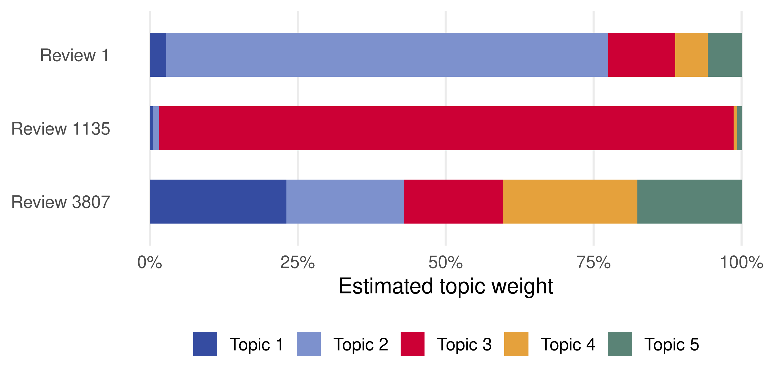
Shown: the first review, the highest topic-3 review, and the most evenly mixed review. These are selected illustrations, not a random sample.
Ratings provide an external comparison
The topic fit used phrase counts alone. We can now compare its weights with the review’s overall rating.
| Overall | Reviews |
|---|---|
| 1 | 615 |
| 2 | 493 |
| 3 | 638 |
| 4 | 1293 |
| 5 | 3127 |
Five-star reviews are the largest group. Different rating groups have different sample sizes.
Waiting-related weight is higher at low ratings
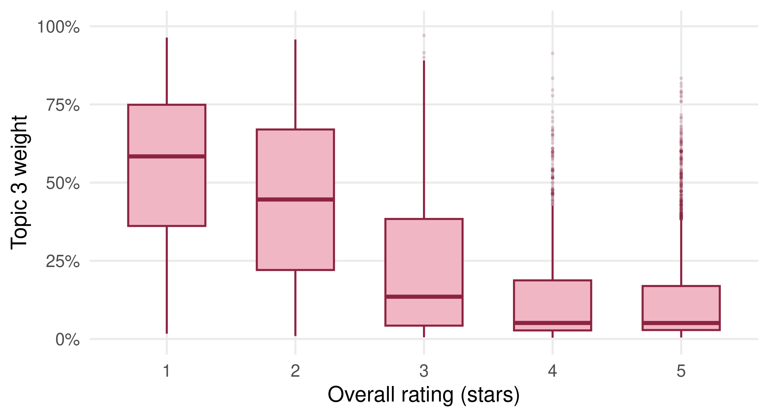
This association supports the tentative label. It does not show that waiting caused the low rating.
Other topics show different rating patterns
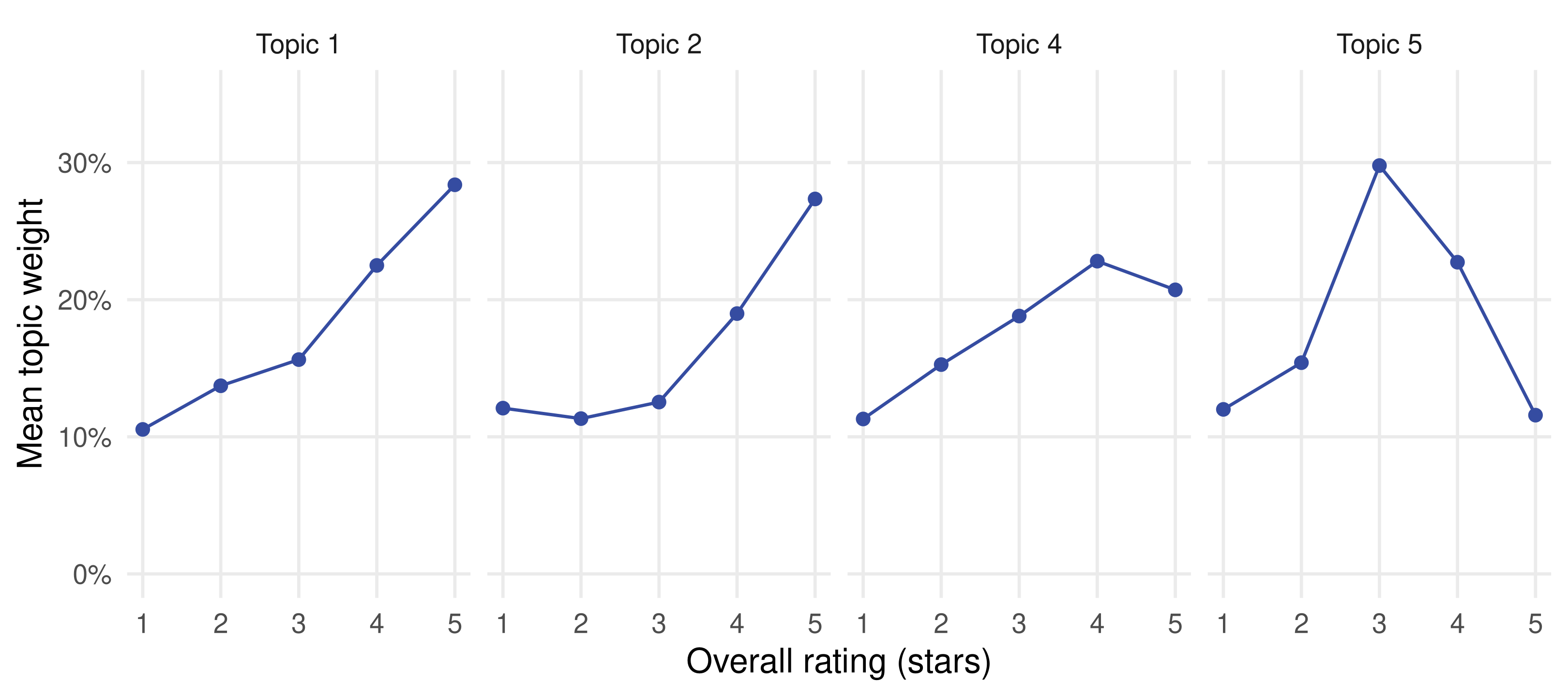
Topics 1 and 2 align with praise; topic 5 peaks at three stars. A topic is not automatically a sentiment score.
Using topics as predictors needs validation
A topic model compresses thousands of token counts into K weights per document.
For prediction on new reviews:
- Split documents before learning the vocabulary and topics.
- Fit topics on training text; infer new documents’ weights using those fitted topics.
- Fit the outcome model on training weights, then evaluate held-out ratings.
Because the K weights sum to one, a regression with an intercept uses K-1 weights or another explicit constraint.
Practice: interpret a topic carefully
Pick one fitted topic other than topic 3.
- Compare five high-probability phrases with five high-lift phrases.
- Propose a label and identify one phrase that challenges it.
- Describe its rating pattern without making a causal claim.
- Explain one check you would make before using it in a research paper.
Text analysis starts with measurement
Define the unit. A speech, a speaker-year, and a review support different questions.
Inspect the representation. Tokenization, pruning, and normalization decide which language survives.
Interpret the model. Regression describes an outcome relationship; topics summarize recurring mixtures.
Validate the claim. Training fit and plausible topic labels are starting points for further evidence.
Reading and data sources
- Silge and Robinson: Text Mining with R — tidy tokenization and analysis.
- Gentzkow and Shapiro (2010) — congressional phrases and media slant.
- Taddy (2013) — the congressional and restaurant examples.
- Gentzkow, Shapiro and Taddy (2019) — historical partisanship in congressional speech.
- Blei, Ng and Jordan (2003) and Taddy (2012) — topic models and estimation.
- Package references:
textir,maptpx,tidytext.
Additional code and model details
Optional examples for practice and reference
Preserve adjacency while cleaning bigrams
bigram_stems <- bigrams %>%
  separate(bigram, into = c("w1", "w2"), sep = " ") %>%
  anti_join(stop_words, by = c("w1" = "word")) %>%
  anti_join(stop_words, by = c("w2" = "word")) %>%
  mutate(across(c(w1, w2),
                ~ SnowballC::wordStem(.x, language = "en"))) %>%
  unite(bigram, w1, w2, sep = " ") %>%
  count(document, bigram, sort = TRUE)
This keeps only originally adjacent pairs. The default stopword rule still discards negation; adjust the list when negation matters.
Retrieve probabilities and lift directly
## # A tibble: 5 × 3
##   phrase      probability  lift
##   <chr>             <dbl> <dbl>
## 1 go back         0.0266   4.38
## 2 first time      0.00874  4.71
## 3 long time       0.00763  4.50
## 4 come back       0.00740  4.44
## 5 even though     0.00630  3.02
Replace desc(probability) with desc(lift) to compare rankings.
Check normalization and row alignment
stopifnot(
  nrow(review_counts) == nrow(ratings),
  identical(rownames(review_counts), rownames(ratings)),
  identical(rownames(tpcs$omega), rownames(review_counts)),
  identical(rownames(tpcs$theta), colnames(review_counts)),
  all(Matrix::rowSums(review_counts) > 0),
  max(abs(colSums(tpcs$theta) - 1)) < 1e-8,
  max(abs(rowSums(tpcs$omega) - 1)) < 1e-8
)
A plot can look plausible even when document rows or vocabulary columns are misaligned.
Compare candidate topic counts
This optional search fits additional models and takes longer.
The package compares approximate log Bayes factors against a one-topic baseline. kill = 0 evaluates every candidate; the default can stop early.
Do not carry the five-topic labels into a newly selected model.
What the MAP fit adds
For document i, the likelihood uses the mixture probability vector
p_i=\sum_{k=1}^{K}\omega_{ik}\theta_k.
maptpx adds Dirichlet priors for both \omega_i and \theta_k, and maximizes the posterior in a logit parametrization.
The prior settings influence how concentrated the estimated distributions are. Different priors, initial values, or K can change the fit.
Predict topic weights for new documents
The new count matrix must use the same vocabulary columns in the same order as the training matrix.
The fitted topic distributions stay fixed; the model estimates weights for each new document. Decide how to handle documents with no retained tokens.
Install the required packages
Run once in your R environment if needed:
Use data("congress109", package = "textir") and data("we8there", package = "textir") to load the bundled examples.
The lecture render uses local package data and does not fetch live research data.
Return to the research question
What is the document? What survives preprocessing? What does the fitted quantity mean?
Those decisions determine which conclusions the analysis can support.