ECON 4370 / 6370 Computing for Economics

Lecture 5: Data Cleaning & Wrangling with Tidyverse

Zhan Gao

10 September 2026

Overview

1. Tidy data
2. Tidyverse basics
3. Data wrangling with dplyr
4. Data tidying with tidyr

Key principles of tidy data

1. Each variable forms a column
2. Each observation forms a row
3. Each type of observational unit forms a table

Basically, tidy data is more likely to be long (i.e. narrow) format than wide format.

The canonical reference is Hadley Wickham’s tidy data paper (2014, Journal of Statistical Software).

Required packages

R packages you’ll need today:

☑ tidyverse

☑ nycflights13

You can install/update them both with the following command:

install.packages(c('tidyverse', 'nycflights13'), repos = 'https://cran.rstudio.com', dependencies = TRUE)

Tidyverse basics

---

Tidyverse vs. base R

Much digital ink has been spilled over the “tidyverse vs. base R” debate.

I won’t delve into this debate here, because I think the answer is clear: We should teach the tidyverse first (or, at least, early).

• The documentation and community support are outstanding
• Having a consistent philosophy and syntax makes it easier to learn
• Provides a convenient “front-end” to big data tools that we’ll use later in the course
• For data cleaning, wrangling, and plotting, the tidyverse really is a no-brainer

Tidyverse vs. base R (cont.)

But… this certainly shouldn’t put you off learning base R alternatives.

• Base R is extremely flexible and powerful (and stable)
• There are some things that you’ll have to venture outside of the tidyverse for
• A combination of tidyverse and base R is often the best solution to a problem

Excellent base R data manipulation tutorials: here and here.

Tidyverse vs. base R (cont.)

One point of convenience is that there is often a direct correspondence between a tidyverse command and its base R equivalent. These generally follow a tidyverse::snake_case vs base::period.case rule:

tidyverse	base
?readr::read_csv	?utils::read.csv
?dplyr::if_else	?base::ifelse
?tibble::tibble	?base::data.frame

The tidyverse alternative typically offers some enhancements or other useful options (and sometimes restrictions) over its base counterpart.

Remember: There are (almost) always multiple ways to achieve a single goal in R.

Tidyverse packages

Let’s load the tidyverse meta-package and check the output:

library(tidyverse)

## ── Attaching core tidyverse packages ──────────────────────── tidyverse 2.0.0 ──
## ✔ dplyr   1.2.1     ✔ readr   2.2.0
## ✔ forcats 1.0.1     ✔ stringr 1.6.0
## ✔ ggplot2 4.0.3     ✔ tibble  3.3.1
## ✔ purrr   1.2.2     ✔ tidyr   1.3.2
## ── Conflicts ────────────────────────────────────────── tidyverse_conflicts() ──
## ✖ dplyr::filter() masks stats::filter()
## ✖ dplyr::lag()    masks stats::lag()
## ℹ Use the conflicted package (<http://conflicted.r-lib.org/>) to force all conflicts to become errors

We have actually loaded a number of packages (which could also be loaded individually): ggplot2, tibble, dplyr, etc.

• We can also see information about the package versions and some namespace conflicts

Tidyverse packages (cont.)

The tidyverse actually comes with a lot more packages than those that are just loaded automatically:¹

tidyverse_packages()

##  [1] "broom"         "conflicted"    "cli"           "dbplyr"       
##  [5] "dplyr"         "dtplyr"        "forcats"       "ggplot2"      
##  [9] "googledrive"   "googlesheets4" "haven"         "hms"          
## [13] "httr"          "jsonlite"      "lubridate"     "magrittr"     
## [17] "modelr"        "pillar"        "purrr"         "ragg"         
## [21] "readr"         "readxl"        "reprex"        "rlang"        
## [25] "rstudioapi"    "rvest"         "stringr"       "tibble"       
## [29] "tidyr"         "xml2"          "tidyverse"

We’ll use several of these additional packages during the remainder of this course.

• E.g. The lubridate package for working with dates
• However, bear in mind that these packages have to be loaded separately

¹ It also includes a lot of dependencies upon installation. This is a matter of some controversy.

Focus for today

I hope to cover most of the tidyverse packages over the length of this course.

Today, however, I’m only really going to focus on two packages:

1. dplyr
2. tidyr

These are the workhorse packages for cleaning and wrangling data. They are thus the ones that you will likely make the most use of.

• Data cleaning and wrangling occupies an inordinate amount of time, no matter where you are in your research career

An aside on pipes: %>%

The tidyverse loads its own pipe operator, denoted %>% — the R analogue of the shell’s |.

Using pipes can dramatically improve the experience of reading and writing code. Compare:

## These next two lines of code do exactly the same thing.
mpg %>%
  filter(manufacturer == "audi") %>%
  group_by(model) %>%
  summarise(hwy_mean = mean(hwy))
summarise(group_by(filter(mpg, manufacturer == "audi"), model), hwy_mean = mean(hwy))

The first version reads from left to right, exactly how I thought of the operations in my head.

• Take this object (mpg), do this (filter), then do this (group_by), etc.

The second version totally inverts this logical order (the final operation comes first!)

• Who wants to read things inside out?

Pipes (cont.)

The piped version of the code is even more readable if we write it over several lines. Here it is again and, this time, I’ll run it for good measure so you can see the output:

mpg %>%
  filter(manufacturer == "audi") %>%
  group_by(model) %>%
  summarise(hwy_mean = mean(hwy))

## # A tibble: 3 × 2
##   model      hwy_mean
##   <chr>         <dbl>
## 1 a4             28.3
## 2 a4 quattro     25.8
## 3 a6 quattro     24

Remember: Using vertical space costs nothing and makes for much more readable/writeable code than cramming things horizontally.

PS: The pipe is originally from the magrittr package (geddit?), which can do some other cool things if you’re inclined to explore.

A further aside on the base R pipe: |>

The magrittr pipe has proven so successful and popular that base R gained its own “native” pipe in version 4.1.0, denoted |>.¹

mtcars |> subset(cyl == 4) |> head(3)

##             mpg cyl  disp hp drat   wt  qsec vs am gear carb
## Datsun 710 22.8   4 108.0 93 3.85 2.32 18.61  1  1    4    1
## Merc 240D  24.4   4 146.7 62 3.69 3.19 20.00  1  0    4    2
## Merc 230   22.8   4 140.8 95 3.92 3.15 22.90  1  0    4    2

Since R 4.2.0 you can also pipe into an arbitrary (named) argument with the underscore placeholder _:

mtcars |> subset(cyl == 4) |> lm(formula = mpg ~ disp, data = _)

## 
## Call:
## lm(formula = mpg ~ disp, data = subset(mtcars, cyl == 4))
## 
## Coefficients:
## (Intercept)         disp  
##     40.8720      -0.1351

¹ That’s a | followed by a >. The native pipe arrived together with other new features, like shorthand “lambda” functions, \(x).

Data wrangling with dplyr

---

Key dplyr verbs

There are five key dplyr verbs that you need to learn:

1. filter: Filter (i.e. subset) rows based on their values
2. arrange: Arrange (i.e. reorder) rows based on their values
3. select: Select (i.e. subset) columns by their names
4. mutate: Create new columns
5. summarise: Collapse multiple rows into a single summary value¹

Let’s practice these commands together using the starwars data frame that comes pre-packaged with dplyr.

¹ summarize with a “z” works too.

1) dplyr::filter

We can chain multiple filter commands with the pipe (%>%), or just separate them within a single filter command using commas:

starwars %>%
  filter(
    species == "Human",
    height >= 190
  )

## # A tibble: 4 × 14
##   name      height  mass hair_color skin_color eye_color birth_year sex   gender
##   <chr>      <int> <dbl> <chr>      <chr>      <chr>          <dbl> <chr> <chr> 
## 1 Darth Va…    202   136 none       white      yellow          41.9 male  mascu…
## 2 Qui-Gon …    193    89 brown      fair       blue            92   male  mascu…
## 3 Dooku        193    80 white      fair       brown          102   male  mascu…
## 4 Bail Pre…    191    NA black      tan        brown           67   male  mascu…
## # ℹ 5 more variables: homeworld <chr>, species <chr>, films <list>,
## #   vehicles <list>, starships <list>

1) dplyr::filter (cont.)

Regular expressions work well too:

starwars %>%
  filter(grepl("Skywalker", name))

## # A tibble: 3 × 14
##   name      height  mass hair_color skin_color eye_color birth_year sex   gender
##   <chr>      <int> <dbl> <chr>      <chr>      <chr>          <dbl> <chr> <chr> 
## 1 Luke Sky…    172    77 blond      fair       blue            19   male  mascu…
## 2 Anakin S…    188    84 blond      fair       blue            41.9 male  mascu…
## 3 Shmi Sky…    163    NA black      fair       brown           72   fema… femin…
## # ℹ 5 more variables: homeworld <chr>, species <chr>, films <list>,
## #   vehicles <list>, starships <list>

1) dplyr::filter (cont.)

A very common filter use case is identifying (or removing) missing data cases:

starwars %>%
  filter(is.na(height))

## # A tibble: 6 × 14
##   name      height  mass hair_color skin_color eye_color birth_year sex   gender
##   <chr>      <int> <dbl> <chr>      <chr>      <chr>          <dbl> <chr> <chr> 
## 1 Arvel Cr…     NA    NA brown      fair       brown             NA male  mascu…
## 2 Finn          NA    NA black      dark       dark              NA male  mascu…
## 3 Rey           NA    NA brown      light      hazel             NA fema… femin…
## 4 Poe Dame…     NA    NA brown      light      brown             NA male  mascu…
## 5 BB8           NA    NA none       none       black             NA none  mascu…
## 6 Captain …     NA    NA none       none       unknown           NA fema… femin…
## # ℹ 5 more variables: homeworld <chr>, species <chr>, films <list>,
## #   vehicles <list>, starships <list>

To remove missing observations, simply use negation: filter(!is.na(height)).

2) dplyr::arrange

starwars %>%
  arrange(birth_year)

## # A tibble: 87 × 14
##    name     height  mass hair_color skin_color eye_color birth_year sex   gender
##    <chr>     <int> <dbl> <chr>      <chr>      <chr>          <dbl> <chr> <chr> 
##  1 Wicket …     88  20   brown      brown      brown            8   male  mascu…
##  2 IG-88       200 140   none       metal      red             15   none  mascu…
##  3 Luke Sk…    172  77   blond      fair       blue            19   male  mascu…
##  4 Leia Or…    150  49   brown      light      brown           19   fema… femin…
##  5 Wedge A…    170  77   brown      fair       hazel           21   male  mascu…
##  6 Plo Koon    188  80   none       orange     black           22   male  mascu…
##  7 Biggs D…    183  84   black      light      brown           24   male  mascu…
##  8 Han Solo    180  80   brown      fair       brown           29   male  mascu…
##  9 Lando C…    177  79   black      dark       brown           31   male  mascu…
## 10 Boba Fe…    183  78.2 black      fair       brown           31.5 male  mascu…
## # ℹ 77 more rows
## # ℹ 5 more variables: homeworld <chr>, species <chr>, films <list>,
## #   vehicles <list>, starships <list>

Note: Arranging on a character-based column (i.e. strings) will sort alphabetically. Try this yourself by arranging according to the “name” column.

2) dplyr::arrange (cont.)

We can also arrange items in descending order using arrange(desc()):

starwars %>%
  arrange(desc(birth_year))

## # A tibble: 87 × 14
##    name     height  mass hair_color skin_color eye_color birth_year sex   gender
##    <chr>     <int> <dbl> <chr>      <chr>      <chr>          <dbl> <chr> <chr> 
##  1 Yoda         66    17 white      green      brown            896 male  mascu…
##  2 Jabba D…    175  1358 <NA>       green-tan… orange           600 herm… mascu…
##  3 Chewbac…    228   112 brown      unknown    blue             200 male  mascu…
##  4 C-3PO       167    75 <NA>       gold       yellow           112 none  mascu…
##  5 Dooku       193    80 white      fair       brown            102 male  mascu…
##  6 Qui-Gon…    193    89 brown      fair       blue              92 male  mascu…
##  7 Ki-Adi-…    198    82 white      pale       yellow            92 male  mascu…
##  8 Finis V…    170    NA blond      fair       blue              91 male  mascu…
##  9 Palpati…    170    75 grey       pale       yellow            82 male  mascu…
## 10 Cliegg …    183    NA brown      fair       blue              82 male  mascu…
## # ℹ 77 more rows
## # ℹ 5 more variables: homeworld <chr>, species <chr>, films <list>,
## #   vehicles <list>, starships <list>

3) dplyr::select

Use commas to select multiple columns out of a data frame. (You can also use “first:last” for consecutive columns). Deselect a column with “-”:

starwars %>%
  select(name:skin_color, species, -height)

## # A tibble: 87 × 5
##    name                mass hair_color    skin_color  species
##    <chr>              <dbl> <chr>         <chr>       <chr>  
##  1 Luke Skywalker        77 blond         fair        Human  
##  2 C-3PO                 75 <NA>          gold        Droid  
##  3 R2-D2                 32 <NA>          white, blue Droid  
##  4 Darth Vader          136 none          white       Human  
##  5 Leia Organa           49 brown         light       Human  
##  6 Owen Lars            120 brown, grey   light       Human  
##  7 Beru Whitesun Lars    75 brown         light       Human  
##  8 R5-D4                 32 <NA>          white, red  Droid  
##  9 Biggs Darklighter     84 black         light       Human  
## 10 Obi-Wan Kenobi        77 auburn, white fair        Human  
## # ℹ 77 more rows

3) dplyr::select (cont.): renaming

You can also rename some (or all) of your selected variables in place:

starwars %>%
  select(alias = name, crib = homeworld, sex = gender)

## # A tibble: 87 × 3
##    alias              crib     sex      
##    <chr>              <chr>    <chr>    
##  1 Luke Skywalker     Tatooine masculine
##  2 C-3PO              Tatooine masculine
##  3 R2-D2              Naboo    masculine
##  4 Darth Vader        Tatooine masculine
##  5 Leia Organa        Alderaan feminine 
##  6 Owen Lars          Tatooine masculine
##  7 Beru Whitesun Lars Tatooine feminine 
##  8 R5-D4              Tatooine masculine
##  9 Biggs Darklighter  Tatooine masculine
## 10 Obi-Wan Kenobi     Stewjon  masculine
## # ℹ 77 more rows

If you just want to rename columns without subsetting them, you can use rename. Try this now by replacing select(...) in the above code chunk with rename(...).

3) dplyr::select (cont.): helpers

The select(contains(PATTERN)) option provides a nice shortcut in relevant cases:

starwars %>%
  select(name, contains("color"))

## # A tibble: 87 × 4
##    name               hair_color    skin_color  eye_color
##    <chr>              <chr>         <chr>       <chr>    
##  1 Luke Skywalker     blond         fair        blue     
##  2 C-3PO              <NA>          gold        yellow   
##  3 R2-D2              <NA>          white, blue red      
##  4 Darth Vader        none          white       yellow   
##  5 Leia Organa        brown         light       brown    
##  6 Owen Lars          brown, grey   light       blue     
##  7 Beru Whitesun Lars brown         light       blue     
##  8 R5-D4              <NA>          white, red  red      
##  9 Biggs Darklighter  black         light       brown    
## 10 Obi-Wan Kenobi     auburn, white fair        blue-gray
## # ℹ 77 more rows

3) dplyr::select (cont.): reordering

The select(..., everything()) option is another useful shortcut if you only want to bring some variable(s) to the “front” of a data frame:

starwars %>%
  select(species, homeworld, everything()) %>%
  head(5)

## # A tibble: 5 × 14
##   species homeworld name           height  mass hair_color skin_color  eye_color
##   <chr>   <chr>     <chr>           <int> <dbl> <chr>      <chr>       <chr>    
## 1 Human   Tatooine  Luke Skywalker    172    77 blond      fair        blue     
## 2 Droid   Tatooine  C-3PO             167    75 <NA>       gold        yellow   
## 3 Droid   Naboo     R2-D2              96    32 <NA>       white, blue red      
## 4 Human   Tatooine  Darth Vader       202   136 none       white       yellow   
## 5 Human   Alderaan  Leia Organa       150    49 brown      light       brown    
## # ℹ 6 more variables: birth_year <dbl>, sex <chr>, gender <chr>, films <list>,
## #   vehicles <list>, starships <list>

Note: The relocate function added in dplyr 1.0.0 has brought a lot more functionality to ordering of columns. See here.

4) dplyr::mutate

You can create new columns from scratch, or (more commonly) as transformations of existing columns:

starwars %>%
  select(name, birth_year) %>%
  mutate(dog_years = birth_year * 7) %>%
  mutate(comment = paste0(name, " is ", dog_years, " in dog years."))

## # A tibble: 87 × 4
##    name               birth_year dog_years comment                              
##    <chr>                   <dbl>     <dbl> <chr>                                
##  1 Luke Skywalker           19        133  Luke Skywalker is 133 in dog years.  
##  2 C-3PO                   112        784  C-3PO is 784 in dog years.           
##  3 R2-D2                    33        231  R2-D2 is 231 in dog years.           
##  4 Darth Vader              41.9      293. Darth Vader is 293.3 in dog years.   
##  5 Leia Organa              19        133  Leia Organa is 133 in dog years.     
##  6 Owen Lars                52        364  Owen Lars is 364 in dog years.       
##  7 Beru Whitesun Lars       47        329  Beru Whitesun Lars is 329 in dog yea…
##  8 R5-D4                    NA         NA  R5-D4 is NA in dog years.            
##  9 Biggs Darklighter        24        168  Biggs Darklighter is 168 in dog year…
## 10 Obi-Wan Kenobi           57        399  Obi-Wan Kenobi is 399 in dog years.  
## # ℹ 77 more rows

4) dplyr::mutate (cont.): order aware

Note: mutate is order aware. So you can chain multiple mutates in a single call:

starwars %>%
  select(name, birth_year) %>%
  mutate(
    dog_years = birth_year * 7, ## Separate with a comma
    comment = paste0(name, " is ", dog_years, " in dog years.")
  )

## # A tibble: 87 × 4
##    name               birth_year dog_years comment                              
##    <chr>                   <dbl>     <dbl> <chr>                                
##  1 Luke Skywalker           19        133  Luke Skywalker is 133 in dog years.  
##  2 C-3PO                   112        784  C-3PO is 784 in dog years.           
##  3 R2-D2                    33        231  R2-D2 is 231 in dog years.           
##  4 Darth Vader              41.9      293. Darth Vader is 293.3 in dog years.   
##  5 Leia Organa              19        133  Leia Organa is 133 in dog years.     
##  6 Owen Lars                52        364  Owen Lars is 364 in dog years.       
##  7 Beru Whitesun Lars       47        329  Beru Whitesun Lars is 329 in dog yea…
##  8 R5-D4                    NA         NA  R5-D4 is NA in dog years.            
##  9 Biggs Darklighter        24        168  Biggs Darklighter is 168 in dog year…
## 10 Obi-Wan Kenobi           57        399  Obi-Wan Kenobi is 399 in dog years.  
## # ℹ 77 more rows

4) dplyr::mutate (cont.): with logic

Boolean, logical and conditional operators all work well with mutate too:

starwars %>%
  select(name, height) %>%
  filter(name %in% c("Luke Skywalker", "Anakin Skywalker")) %>%
  mutate(tall1 = height > 180) %>%
  mutate(tall2 = ifelse(height > 180, "Tall", "Short")) ## Same effect, but can choose labels

## # A tibble: 2 × 4
##   name             height tall1 tall2
##   <chr>             <int> <lgl> <chr>
## 1 Luke Skywalker      172 FALSE Short
## 2 Anakin Skywalker    188 TRUE  Tall

4) dplyr::mutate (cont.): across

Combining mutate with the across feature in dplyr 1.0.0+ allows you to easily work on a subset of variables. For example:

starwars %>%
  select(name:eye_color) %>%
  mutate(across(where(is.character), toupper)) %>% # convert all character variables to uppercase
  head(5)

## # A tibble: 5 × 6
##   name           height  mass hair_color skin_color  eye_color
##   <chr>           <int> <dbl> <chr>      <chr>       <chr>    
## 1 LUKE SKYWALKER    172    77 BLOND      FAIR        BLUE     
## 2 C-3PO             167    75 <NA>       GOLD        YELLOW   
## 3 R2-D2              96    32 <NA>       WHITE, BLUE RED      
## 4 DARTH VADER       202   136 NONE       WHITE       YELLOW   
## 5 LEIA ORGANA       150    49 BROWN      LIGHT       BROWN

Note: This workflow (i.e. combining mutate and across) supersedes the old “scoped” variants of mutate that you might have seen previously. More details here and here.

5) dplyr::summarise

Particularly useful in combination with the group_by command:

starwars %>%
  group_by(species, gender) %>%
  summarise(mean_height = mean(height, na.rm = TRUE))

## # A tibble: 42 × 3
## # Groups:   species [38]
##    species   gender    mean_height
##    <chr>     <chr>           <dbl>
##  1 Aleena    masculine          79
##  2 Besalisk  masculine         198
##  3 Cerean    masculine         198
##  4 Chagrian  masculine         196
##  5 Clawdite  feminine          168
##  6 Droid     feminine           96
##  7 Droid     masculine         140
##  8 Dug       masculine         112
##  9 Ewok      masculine          88
## 10 Geonosian masculine         183
## # ℹ 32 more rows

5) dplyr::summarise (cont.): na.rm

Note that including na.rm = TRUE is usually a good idea with summarise functions. Otherwise, any missing value will propagate to the summarised value too:

## Probably not what we want
starwars %>%
  summarise(mean_height = mean(height))

## # A tibble: 1 × 1
##   mean_height
##         <dbl>
## 1          NA

## Much better
starwars %>%
  summarise(mean_height = mean(height, na.rm = TRUE))

## # A tibble: 1 × 1
##   mean_height
##         <dbl>
## 1        175.

5) dplyr::summarise (cont.): across

The same across-based workflow that we saw with mutate a few slides back also works with summarise. For example:

starwars %>%
  group_by(species) %>%
  summarise(across(where(is.numeric), \(x) mean(x, na.rm = TRUE))) %>%
  head(5)

## # A tibble: 5 × 4
##   species  height  mass birth_year
##   <chr>     <dbl> <dbl>      <dbl>
## 1 Aleena       79    15        NaN
## 2 Besalisk    198   102        NaN
## 3 Cerean      198    82         92
## 4 Chagrian    196   NaN        NaN
## 5 Clawdite    168    55        NaN

Note: \(x) mean(x, na.rm = TRUE) is an anonymous (“lambda”) function. Supplying extra arguments through across(..., mean, na.rm = TRUE) was deprecated in dplyr 1.1.0.

Other dplyr goodies

group_by and ungroup: For (un)grouping.

• Particularly useful with the summarise and mutate commands, as we’ve already seen

slice: Subset rows by position rather than filtering by values.

• E.g. starwars %>% slice(c(1, 5))

pull: Extract a column from a data frame as a vector or scalar.

• E.g. starwars %>% filter(gender=="feminine") %>% pull(height)

Other dplyr goodies (cont.)

count and distinct: Number and isolate unique observations.

• E.g. starwars %>% count(species), or starwars %>% distinct(species)
• You could also use a combination of mutate, group_by, and n(), e.g. starwars %>% group_by(species) %>% mutate(num = n())

There is also a whole class of window functions for getting leads and lags, ranking, creating cumulative aggregates, etc.

• See vignette("window-functions")

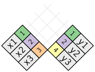
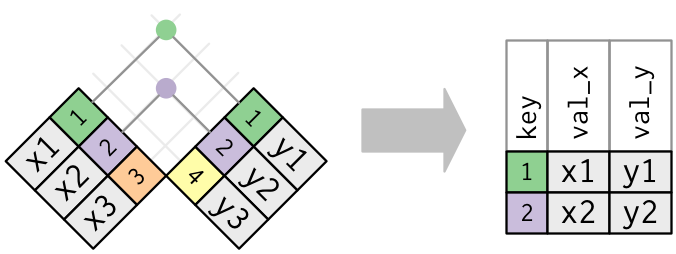
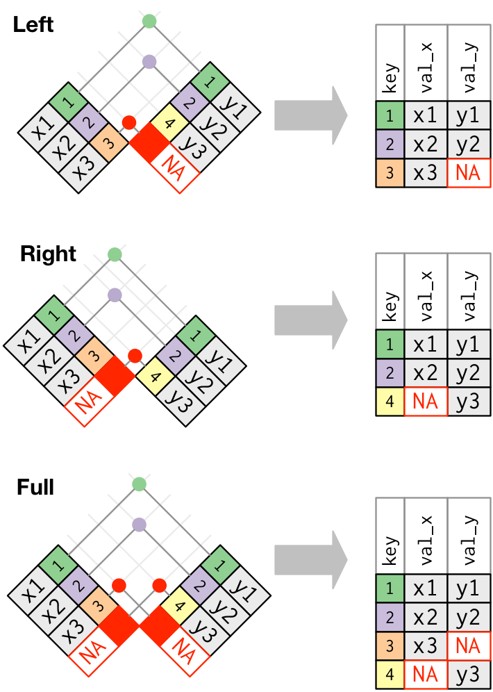
The final set of dplyr “goodies” are the family of join operations. These are important enough that I want to go over some concepts in a bit more depth…

• We will encounter and practice these many more times as the course progresses

Joins: relational data

In real-world data analysis, information is often spread across multiple tables or datasets, i.e. we often encounter relational data, where we have multiple tables that are related to each other.

For the simple examples that I’m going to show here, we’ll need some data sets that come bundled with the nycflights13 package:

library(nycflights13)

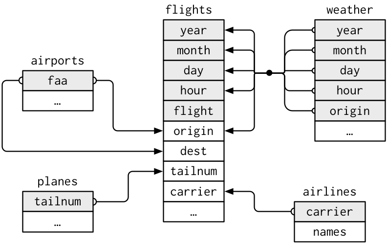
nycflights13 contains four tibbles that are related to the flights table: airlines, airports, planes, and weather.

The related tables: airlines

airlines lets you look up the full carrier name from its abbreviated code:

airlines

## # A tibble: 16 × 2
##    carrier name                       
##    <chr>   <chr>                      
##  1 9E      Endeavor Air Inc.          
##  2 AA      American Airlines Inc.     
##  3 AS      Alaska Airlines Inc.       
##  4 B6      JetBlue Airways            
##  5 DL      Delta Air Lines Inc.       
##  6 EV      ExpressJet Airlines Inc.   
##  7 F9      Frontier Airlines Inc.     
##  8 FL      AirTran Airways Corporation
##  9 HA      Hawaiian Airlines Inc.     
## 10 MQ      Envoy Air                  
## 11 OO      SkyWest Airlines Inc.      
## 12 UA      United Air Lines Inc.      
## 13 US      US Airways Inc.            
## 14 VX      Virgin America             
## 15 WN      Southwest Airlines Co.     
## 16 YV      Mesa Airlines Inc.

The related tables: airports

airports gives information about each airport, identified by the faa airport code:

airports

## # A tibble: 1,458 × 8
##    faa   name                             lat    lon   alt    tz dst   tzone    
##    <chr> <chr>                          <dbl>  <dbl> <dbl> <dbl> <chr> <chr>    
##  1 04G   Lansdowne Airport               41.1  -80.6  1044    -5 A     America/…
##  2 06A   Moton Field Municipal Airport   32.5  -85.7   264    -6 A     America/…
##  3 06C   Schaumburg Regional             42.0  -88.1   801    -6 A     America/…
##  4 06N   Randall Airport                 41.4  -74.4   523    -5 A     America/…
##  5 09J   Jekyll Island Airport           31.1  -81.4    11    -5 A     America/…
##  6 0A9   Elizabethton Municipal Airport  36.4  -82.2  1593    -5 A     America/…
##  7 0G6   Williams County Airport         41.5  -84.5   730    -5 A     America/…
##  8 0G7   Finger Lakes Regional Airport   42.9  -76.8   492    -5 A     America/…
##  9 0P2   Shoestring Aviation Airfield    39.8  -76.6  1000    -5 U     America/…
## 10 0S9   Jefferson County Intl           48.1 -123.    108    -8 A     America/…
## # ℹ 1,448 more rows

The related tables: planes

planes contains information about each plane, identified by the tailnum plane code:

planes

## # A tibble: 3,322 × 9
##    tailnum  year type              manufacturer model engines seats speed engine
##    <chr>   <int> <chr>             <chr>        <chr>   <int> <int> <int> <chr> 
##  1 N10156   2004 Fixed wing multi… EMBRAER      EMB-…       2    55    NA Turbo…
##  2 N102UW   1998 Fixed wing multi… AIRBUS INDU… A320…       2   182    NA Turbo…
##  3 N103US   1999 Fixed wing multi… AIRBUS INDU… A320…       2   182    NA Turbo…
##  4 N104UW   1999 Fixed wing multi… AIRBUS INDU… A320…       2   182    NA Turbo…
##  5 N10575   2002 Fixed wing multi… EMBRAER      EMB-…       2    55    NA Turbo…
##  6 N105UW   1999 Fixed wing multi… AIRBUS INDU… A320…       2   182    NA Turbo…
##  7 N107US   1999 Fixed wing multi… AIRBUS INDU… A320…       2   182    NA Turbo…
##  8 N108UW   1999 Fixed wing multi… AIRBUS INDU… A320…       2   182    NA Turbo…
##  9 N109UW   1999 Fixed wing multi… AIRBUS INDU… A320…       2   182    NA Turbo…
## 10 N110UW   1999 Fixed wing multi… AIRBUS INDU… A320…       2   182    NA Turbo…
## # ℹ 3,312 more rows

The related tables: weather

weather contains information about the weather at each airport for each hour:

weather

## # A tibble: 26,115 × 15
##    origin  year month   day  hour  temp  dewp humid wind_dir wind_speed
##    <chr>  <int> <int> <int> <int> <dbl> <dbl> <dbl>    <dbl>      <dbl>
##  1 EWR     2013     1     1     1  39.0  26.1  59.4      270      10.4 
##  2 EWR     2013     1     1     2  39.0  27.0  61.6      250       8.06
##  3 EWR     2013     1     1     3  39.0  28.0  64.4      240      11.5 
##  4 EWR     2013     1     1     4  39.9  28.0  62.2      250      12.7 
##  5 EWR     2013     1     1     5  39.0  28.0  64.4      260      12.7 
##  6 EWR     2013     1     1     6  37.9  28.0  67.2      240      11.5 
##  7 EWR     2013     1     1     7  39.0  28.0  64.4      240      15.0 
##  8 EWR     2013     1     1     8  39.9  28.0  62.2      250      10.4 
##  9 EWR     2013     1     1     9  39.9  28.0  62.2      260      15.0 
## 10 EWR     2013     1     1    10  41    28.0  59.6      260      13.8 
## # ℹ 26,105 more rows
## # ℹ 5 more variables: wind_gust <dbl>, precip <dbl>, pressure <dbl>,
## #   visib <dbl>, time_hour <dttm>

How the tables relate

To analyze the data, for instance, we might want to:

• Add airline names to make our analysis more readable (flights + airlines)
• Include weather conditions to study flight delays (flights + weather)
• Analyze aircraft characteristics and their impact on performance (flights + planes)

We need to combine (join) the data from these tables to answer more complex questions.

Keys and values

To help visualize the idea, think about the canonical example of a database table:

• The coloured column represents the “key” variable: these are used to match the rows between the tables.
• The grey column represents the “value” column that is carried along for the ride.
• In these examples I’ll show a single key variable, but the idea generalises in a straightforward way to multiple keys and multiple values.

Join operations: inner join

One of the mainstays of the dplyr package is merging data with the family of join operations.

• inner_join(df1, df2): Returns only rows that have matching values in both data frames.

Join operations: outer joins

Outer joins keep observations that appear in at least one of the tables:

• left_join(df1, df2): Returns all rows from the left data frame and matching rows from the right.
• right_join(df1, df2): Returns all rows from the right data frame and matching rows from the left.
• full_join(df1, df2): Returns all rows from both data frames, filling in missing values with NA.

Join operations: filtering joins

• semi_join(df1, df2): Returns rows from the left data frame that have a match in the right data frame.

• anti_join(df1, df2): Returns rows from the left data frame that do not have a match in the right data frame.

Practice: join flights and planes

Let’s perform a left join on the flights and planes datasets:

left_join(flights, planes) %>%
  select(year, month, day, dep_time, arr_time, carrier, flight, tailnum, type, model)

## Joining with `by = join_by(year, tailnum)`

## # A tibble: 336,776 × 10
##     year month   day dep_time arr_time carrier flight tailnum type  model
##    <int> <int> <int>    <int>    <int> <chr>    <int> <chr>   <chr> <chr>
##  1  2013     1     1      517      830 UA        1545 N14228  <NA>  <NA> 
##  2  2013     1     1      533      850 UA        1714 N24211  <NA>  <NA> 
##  3  2013     1     1      542      923 AA        1141 N619AA  <NA>  <NA> 
##  4  2013     1     1      544     1004 B6         725 N804JB  <NA>  <NA> 
##  5  2013     1     1      554      812 DL         461 N668DN  <NA>  <NA> 
##  6  2013     1     1      554      740 UA        1696 N39463  <NA>  <NA> 
##  7  2013     1     1      555      913 B6         507 N516JB  <NA>  <NA> 
##  8  2013     1     1      557      709 EV        5708 N829AS  <NA>  <NA> 
##  9  2013     1     1      557      838 B6          79 N593JB  <NA>  <NA> 
## 10  2013     1     1      558      753 AA         301 N3ALAA  <NA>  <NA> 
## # ℹ 336,766 more rows

Practice: join flights and planes (cont.)

Note that dplyr made a reasonable guess about which columns to join on (i.e. columns that share the same name). It also told us its choices in a message:

## Joining with `by = join_by(year, tailnum)`

However, there’s an obvious problem here: the variable “year” does not have a consistent meaning across our joining datasets!

• In one it refers to the year of flight, in the other it refers to year of construction

That is why we see so many NAs in the type and model columns on the previous slide: rows only match if both year and tailnum agree.

Be specific with by =

Luckily, there’s an easy way to avoid this problem. You just need to be more explicit in your join call by using the by = argument. You can also rename any ambiguous columns to avoid confusion:

left_join(
  flights,
  planes %>% rename(year_built = year), ## Not necessary w/ below line, but helpful
  by = "tailnum" ## Be specific about the joining column
) %>%
  select(year, month, day, dep_time, arr_time, carrier, flight, tailnum, year_built, type, model) %>%
  head(3) ## Just to save space on the slide

## # A tibble: 3 × 11
##    year month   day dep_time arr_time carrier flight tailnum year_built type    
##   <int> <int> <int>    <int>    <int> <chr>    <int> <chr>        <int> <chr>   
## 1  2013     1     1      517      830 UA        1545 N14228        1999 Fixed w…
## 2  2013     1     1      533      850 UA        1714 N24211        1998 Fixed w…
## 3  2013     1     1      542      923 AA        1141 N619AA        1990 Fixed w…
## # ℹ 1 more variable: model <chr>

What if we don’t rename?

Note what happens if we again specify the join column… but do not rename the ambiguous “year” column in at least one of the given data frames:

left_join(
  flights,
  planes, ## Not renaming "year" to "year_built" this time
  by = "tailnum"
) %>%
  select(contains("year"), month, day, dep_time, arr_time, carrier, flight, tailnum, type, model) %>%
  head(3)

## # A tibble: 3 × 11
##   year.x year.y month   day dep_time arr_time carrier flight tailnum type  model
##    <int>  <int> <int> <int>    <int>    <int> <chr>    <int> <chr>   <chr> <chr>
## 1   2013   1999     1     1      517      830 UA        1545 N14228  Fixe… 737-…
## 2   2013   1998     1     1      533      850 UA        1714 N24211  Fixe… 737-…
## 3   2013   1990     1     1      542      923 AA        1141 N619AA  Fixe… 757-…

Make sure you know what “year.x” and “year.y” are. Again, it pays to be specific.

Data tidying with tidyr

---

Key tidyr verbs

1. pivot_longer: Pivot wide data into long format (i.e. “melt”)¹
2. pivot_wider: Pivot long data into wide format (i.e. “cast”)²
3. separate: Separate (i.e. split) one column into multiple columns
4. unite: Unite (i.e. combine) multiple columns into one

• Side question: Which of pivot_longer vs pivot_wider produces “tidy” data?

¹ Updated version of tidyr::gather. ² Updated version of tidyr::spread.

1) tidyr::pivot_longer

stocks <- data.frame( ## Could use "tibble" instead of "data.frame" if you prefer
  time = as.Date("2009-01-01") + 0:1,
  X = runif(2, 0, 1),
  Y = runif(2, 0, 2),
  Z = runif(2, 0, 4)
)
stocks

##         time          X         Y        Z
## 1 2009-01-01 0.20995114 0.2391195 3.287572
## 2 2009-01-02 0.06887042 1.2497693 2.846810

stocks %>% pivot_longer(-time, names_to = "stock", values_to = "price")

## # A tibble: 6 × 3
##   time       stock  price
##   <date>     <chr>  <dbl>
## 1 2009-01-01 X     0.210 
## 2 2009-01-01 Y     0.239 
## 3 2009-01-01 Z     3.29  
## 4 2009-01-02 X     0.0689
## 5 2009-01-02 Y     1.25  
## 6 2009-01-02 Z     2.85

2) tidyr::pivot_wider

Let’s quickly save the “tidy” (i.e. long) stocks data frame, then pivot it back to wide:

## Write out the argument names this time: i.e. "names_to=" and "values_to="
tidy_stocks <-
  stocks %>%
  pivot_longer(-time, names_to = "stock", values_to = "price")

tidy_stocks %>% pivot_wider(names_from = stock, values_from = price)

## # A tibble: 2 × 4
##   time           X     Y      Z
##   <date>     <dbl> <dbl>  <dbl>
## 1 2009-01-01 0.391 0.622 -0.756
## 2 2009-01-02 0.151 1.19  -4.11

tidy_stocks %>% pivot_wider(names_from = time, values_from = price)

## # A tibble: 3 × 3
##   stock `2009-01-01` `2009-01-02`
##   <chr>        <dbl>        <dbl>
## 1 X            0.391        0.151
## 2 Y            0.622        1.19 
## 3 Z           -0.756       -4.11

Note that the second example, which used a different combination of pivoting arguments, has effectively transposed the data.

Aside: remembering the pivot_* syntax

There’s a long-running joke about no-one being able to remember Stata’s “reshape” command. (Exhibit A.)

It’s easy to see this happening with the pivot_* functions too. However, I find that I never forget the commands as long as I remember the argument order is “names” then “values”.

3) tidyr::separate

economists <- data.frame(name = c("Adam.Smith", "Paul.Samuelson", "Milton.Friedman"))
economists

##              name
## 1      Adam.Smith
## 2  Paul.Samuelson
## 3 Milton.Friedman

economists %>% separate(name, c("first_name", "last_name"))

##   first_name last_name
## 1       Adam     Smith
## 2       Paul Samuelson
## 3     Milton  Friedman

This command is pretty smart. But to avoid ambiguity, you can also specify the separation character. Note that sep is interpreted as a regular expression, so a literal dot must be escaped: separate(..., sep = "\\.").

3) tidyr::separate_rows

A related function is separate_rows, for splitting up cells that contain multiple fields or observations (a frustratingly common occurrence with survey data):

jobs <- data.frame(
  name = c("Jack", "Jill"),
  occupation = c("Homemaker", "Philosopher, Philanthropist, Troublemaker")
)
jobs

##   name                                occupation
## 1 Jack                                 Homemaker
## 2 Jill Philosopher, Philanthropist, Troublemaker

## Now split out Jill's various occupations into different rows
jobs %>% separate_rows(occupation)

## # A tibble: 4 × 2
##   name  occupation    
##   <chr> <chr>         
## 1 Jack  Homemaker     
## 2 Jill  Philosopher   
## 3 Jill  Philanthropist
## 4 Jill  Troublemaker

4) tidyr::unite

gdp <- data.frame(
  yr = rep(2016, times = 4),
  mnth = rep(1, times = 4),
  dy = 1:4,
  gdp = rnorm(4, mean = 100, sd = 2)
)
gdp

##     yr mnth dy       gdp
## 1 2016    1  1  99.64554
## 2 2016    1  2 101.02705
## 3 2016    1  3 101.00269
## 4 2016    1  4 101.67986

## Combine "yr", "mnth", and "dy" into one "date" column
gdp %>% unite(date, c("yr", "mnth", "dy"), sep = "-")

##       date       gdp
## 1 2016-1-1  99.64554
## 2 2016-1-2 101.02705
## 3 2016-1-3 101.00269
## 4 2016-1-4 101.67986

4) tidyr::unite (cont.)

Note that unite will automatically create a character variable. You can see this better if we convert it to a tibble:

gdp_u <- gdp %>%
  unite(date, c("yr", "mnth", "dy"), sep = "-") %>%
  as_tibble()
gdp_u

## # A tibble: 4 × 2
##   date       gdp
##   <chr>    <dbl>
## 1 2016-1-1  99.6
## 2 2016-1-2 101. 
## 3 2016-1-3 101. 
## 4 2016-1-4 102.

If you want to convert it to something else (e.g. date or numeric) then you will need to modify it using mutate, e.g. with the lubridate package’s super helpful date conversion functions:

library(lubridate)
gdp_u %>% mutate(date = ymd(date))

## # A tibble: 4 × 2
##   date         gdp
##   <date>     <dbl>
## 1 2016-01-01  99.6
## 2 2016-01-02 101. 
## 3 2016-01-03 101. 
## 4 2016-01-04 102.

Other tidyr goodies

Use crossing to get the full combination of a group of variables:¹

crossing(side = c("left", "right"), height = c("top", "bottom"))

## # A tibble: 4 × 2
##   side  height
##   <chr> <chr> 
## 1 left  bottom
## 2 left  top   
## 3 right bottom
## 4 right top

See ?expand and ?complete for more specialised functions that allow you to fill in (implicit) missing data or variable combinations in existing data frames.

¹ Base R alternative: expand.grid.

Resources

• Vignette (from the tidyr package)
• Original paper (Hadley Wickham, 2014 JSS)
• R for Data Science