ECO 4354/6354 — Study Guide and Some Practice Problems for Test 1
Guidelines
- The best way to prepare for the exam is to review the lecture slides and make sure you understand the concepts.
- The coverage of the exam spans the following topics:
- Linear regression models
- Basic concepts of forecasting
- Trend and seasonality
- Covariance stationary process
- Autoregresion models
- The following questions help you get a sense of the calculation type questions possibly in the exam.
An AR(1) with an intercept
Let \[ y_t = 4 + 0.8\, y_{t-1} + \varepsilon_t, \qquad \varepsilon_t \sim WN(0, \sigma^2) \text{ with } \sigma^2 = 3.6, \] and suppose \(\{y_t\}\) is covariance stationary.
- Calculate the unconditional mean \(E(y_t)\).
- Calculate \(\gamma(0)\), \(\gamma(1)\) and \(\gamma(2)\), and then \(\rho(2)\) and \(p(2)\).
- Calculate \(\operatorname{Var}(y_t \mid y_{t-1})\) and compare it with \(\gamma(0)\). By what factor does knowing last period’s value reduce the uncertainty about \(y_t\), and what would that factor be if \(\phi\) were \(0.95\)?
- Does the intercept change any of the autocovariances? Explain in one sentence.
An AR(2)
Let \[ y_t = 0.6\, y_{t-1} + 0.2\, y_{t-2} + \varepsilon_t, \qquad \varepsilon_t \sim WN(0, \sigma^2) \text{ with } \sigma^2 = 2.1 , \] and suppose \(\{y_t\}\) is covariance stationary.
- Calculate \(\rho(1)\), \(\rho(2)\) and \(\rho(3)\).
- Calculate \(\gamma(0)\), \(\gamma(1)\) and \(\gamma(2)\). (Work out the autocorrelations first and use the Yule-Walker equation at \(\tau = 0\).)
- Write down \(p(1)\), \(p(2)\) and \(p(3)\), with a one-line justification for each.
Yuke-Walker equations
Let \(\{y_t\}\) be a covariance stationary AR(2) process with zero mean, and suppose its first three autocovariances are \[ \gamma(0) = 4, \qquad \gamma(1) = 2, \qquad \gamma(2) = 1.6 . \]
- Find \(\phi_1\) and \(\phi_2\). (Write the Yule-Walker equations at \(\tau = 1\) and \(\tau = 2\) and solve the two linear equations in \(\phi_1\) and \(\phi_2\).)
- Find \(\sigma^2\), the variance of the innovation.
- Find \(\gamma(3)\).
- Verify that the process you have recovered is covariance stationary.
Check Stationarity
Let \(\{y_t\}\) have \(E(y_t) = \mu\) for all \(t\), and let \(\gamma(t, \tau) = \operatorname{Cov}(y_t, y_{t-\tau})\) for all dates \(t\) and all displacements \(\tau = 0, 1, 2, \ldots\), so that \(\gamma(t, 0) = \operatorname{Var}(y_t)\). Which of the following candidate autocovariance functions are consistent with covariance stationarity, and which are not? Briefly explain why for each.
- \(\gamma(t, \tau) = 2 \cdot (0.6)^{\tau}\)
- \(\gamma(t, \tau) = 3 + \tau\)
- \(\gamma(t, \tau) = (0.9)^{t} \cdot (0.5)^{\tau}\)
- \(\gamma(t, \tau) = \dfrac{1}{1 + \tau}\)
Check Stationarity II
For each of the following, \(\varepsilon_t \sim \text{iid } N(0, \sigma^2)\) with \(0 < \sigma^2 < \infty\). Decide whether the process is covariance stationary, and name the requirement that fails when it is not.
- \(y_t = 0.5 + 0.9\, y_{t-1} + \varepsilon_t\), started in the indefinite past.
- \(y_t = y_{t-1} + \varepsilon_t\), with \(y_0 = 0\).
- \(y_t = 0.02\, t + \varepsilon_t\).
- \(y_t = \varepsilon_t\) when \(t\) is odd and \(y_t = 2\, \varepsilon_t\) when \(t\) is even.
Check Starionarity III
For each of the following processes, \(\varepsilon_t \sim WN(0, 2)\). Determine whether \(\{y_t\}\) is covariance stationary, and justify your answer with the roots of the autoregressive lag polynomial.
- \(y_t = 1.2\, y_{t-1} - 0.32\, y_{t-2} + \varepsilon_t\)
- \(y_t = 0.2\, y_{t-1} + 0.8\, y_{t-2} + \varepsilon_t\)
- \(y_t = 0.8\, y_{t-1} - 0.25\, y_{t-2} + \varepsilon_t\)
- \(y_t = 1.75\, y_{t-1} - 0.625\, y_{t-2} + \varepsilon_t\)
Reading a correlogram
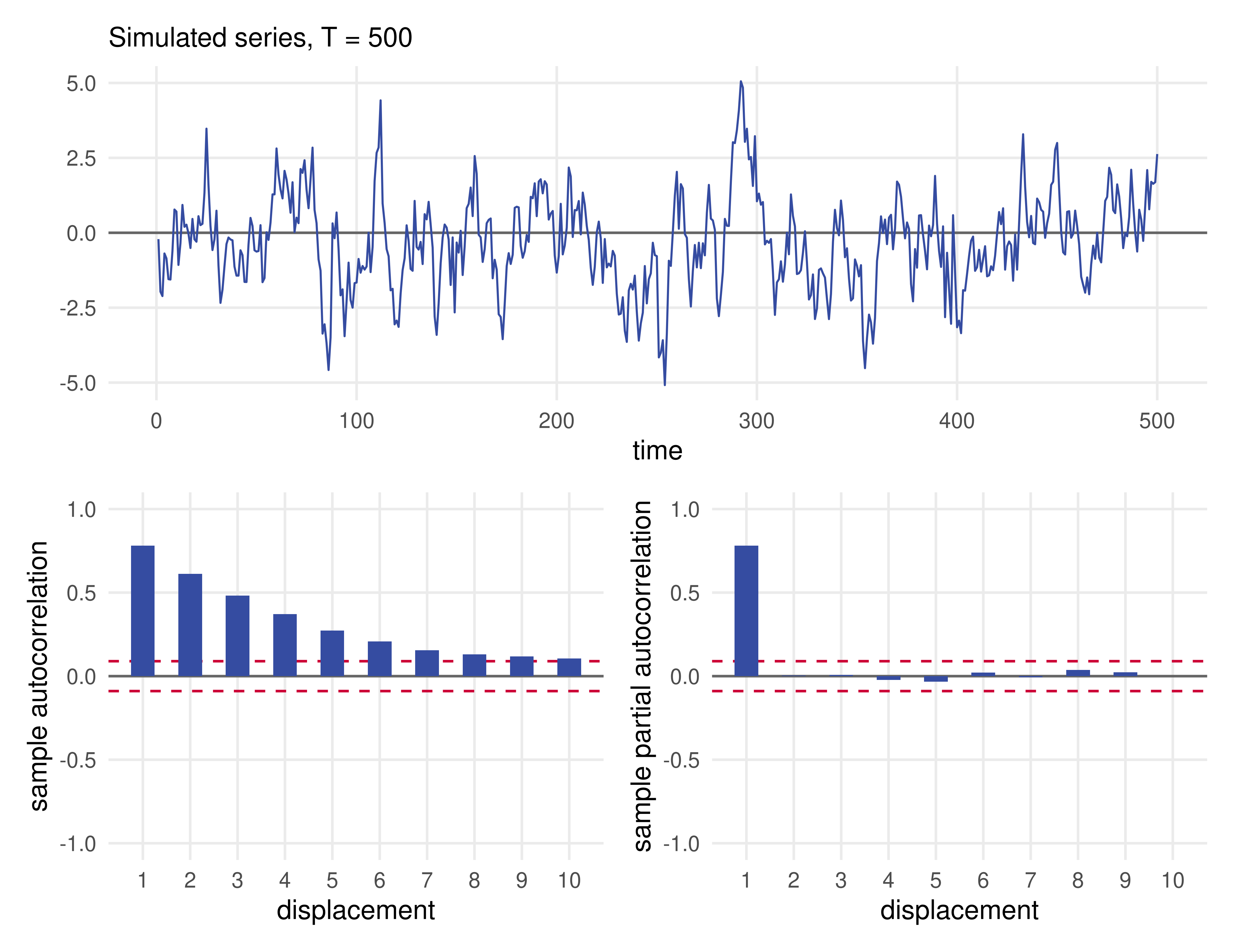
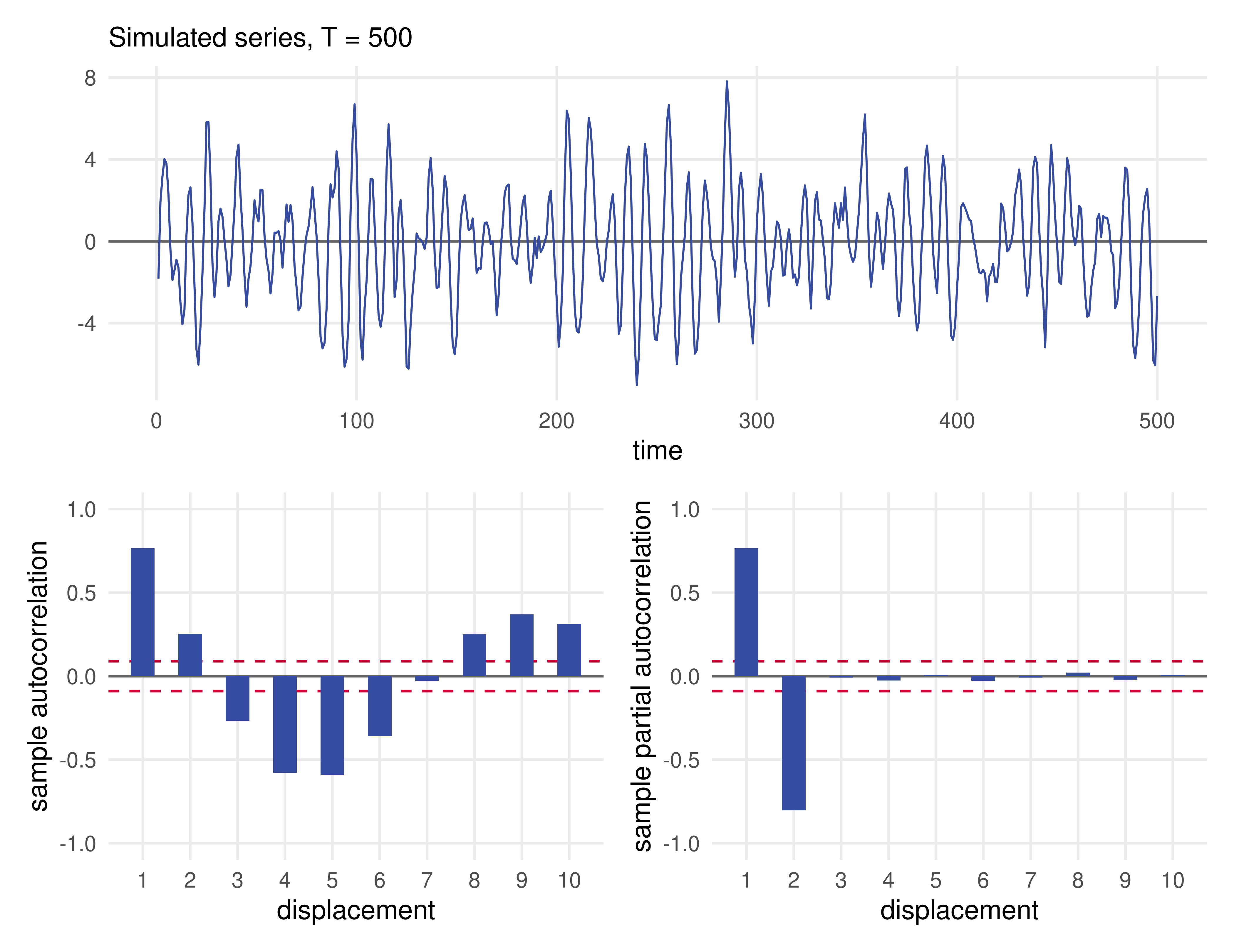
Each series was generated by one of the following models:
The menu. (A) white noise; (B) AR(1); (C) AR(2); (D) AR(3); (E) AR(4).
For each figure, state which model generated the series and explain your reasoning by pointing to specific features of the two correlograms.
Figure 1
Figure 2