# E: matrix of forecast errors, one column per forecast
bg_weights <- function(E) { S <- cov(E); w <- solve(S, rep(1, ncol(E))); w / sum(w) }ECON 4354 / 6354 Forecasting
Lecture 13: Forecast Combination
Zhan Gao
02 October 2026
After the horse race
In the forecast evaluation lecture we learned to tell a better forecast from a lucky one. A horse race ends with a winner, and the natural next step is to discard the losers.
Almost always a mistake. Two forecasts that are each imperfect usually err in different ways, and a weighted average of them is then more accurate than either. This is forecast combination (Bates and Granger, 1969): the forecasting counterpart of a diversified portfolio.
Today: when combining can help (encompassing), how to choose the weights (variance-covariance and regression methods), why equal weights are so hard to beat, two applications (the shipping forecasts and GDP growth), and the largest combination machines in economics, the surveys of forecasters.
Roadmap
Diebold, Forecasting in Economics, Business, Finance and Beyond, the chapters on model-based and on survey-based forecast combination. Data: the OverSea Shipping forecasts of the evaluation lecture and the Survey of Professional Forecasters.
Forecast encompassing: when combination can help
Does one forecast contain the other?
Two forecasts of the same object, y_{a,t+h,t} and y_{b,t+h,t}. Regress the realization on both:
y_{t+h} = \beta_a\, y_{a,t+h,t} + \beta_b\, y_{b,t+h,t} + \varepsilon_{t+h,t} .
- If (\beta_a, \beta_b) = (1, 0), forecast a encompasses forecast b: b adds nothing once a is known.
- If (\beta_a, \beta_b) = (0, 1), b encompasses a.
- For any other pair, neither encompasses the other: both contain useful information, and combining them is potentially desirable.
In covariance stationary environments the encompassing hypotheses are tested with the usual tools, with HAC standard errors or MA(h-1) disturbances when h > 1. Failure of each forecast to encompass the other says that both models are misspecified, which, for intentional abstractions of a complex reality, is the normal state of affairs.
Chong and Hendry (1986) and Fair and Shiller (1990) formalized the idea; the regression is the Mincer-Zarnowitz regression with two forecasts.
Combine information, or combine forecasts?
If information sets could be pooled instantly and costlessly, there would be no role for combining forecasts: build one model on the union of the information and it would encompass all the others.
In the short run that is rarely possible. Deadlines must be met, the other forecaster’s model and data are not available, and the judgment behind a survey response cannot be written down. So we take the forecasts as the primitives and combine them, because we cannot combine what produced them.
Combination is thus the link between two processes: the real-time production of forecasts, where pooling forecasts is all we can do, and the longer-run development of models, where a persistent failure to encompass tells us what to learn from the competitors.
Hence also the appeal of surveys and markets: they combine information sets that no single modeler has.
Variance-covariance combination
Two unbiased forecasts with uncorrelated errors
Take the convex combination y_C = \lambda\, y_a + (1 - \lambda)\, y_b with \lambda \in [0, 1]. The error inherits the weights,
e_C = y - y_C = \lambda\, e_a + (1 - \lambda)\, e_b ,
so if y_a and y_b are unbiased so is y_C, and minimizing MSE means minimizing the error variance.
With uncorrelated errors, \sigma_C^2 = \lambda^2 \sigma_a^2 + (1 - \lambda)^2 \sigma_b^2. Setting the derivative to zero,
\lambda^* = \frac{\sigma_b^2}{\sigma_a^2 + \sigma_b^2} = \frac{1}{1 + \phi^2}, \qquad \phi = \frac{\sigma_a}{\sigma_b} .
- The more accurate forecast gets the larger weight, and the weights are governed by the ratio of error standard deviations: \phi \to 0 gives \lambda^* \to 1, \phi \to \infty gives \lambda^* \to 0.
- Equal accuracy, \phi = 1, gives \lambda^* = 1/2, and then \sigma_C^2 = \sigma_a^2 / 2: half the error variance of either forecast, for free.
Nothing forces \lambda \in [0,1], but weights outside it would be unusual for two sensible forecasts.
Correlated errors
In practice forecast errors are positively correlated: forecasters share information and shocks. With \sigma_{ab} = \operatorname{cov}(e_a, e_b) and \rho = \operatorname{corr}(e_a, e_b),
\sigma_C^2 = \lambda^2 \sigma_a^2 + (1-\lambda)^2 \sigma_b^2 + 2\lambda(1-\lambda)\sigma_{ab} \quad\Longrightarrow\quad \lambda^* = \frac{\sigma_b^2 - \sigma_{ab}}{\sigma_a^2 + \sigma_b^2 - 2\sigma_{ab}} = \frac{1 - \phi\rho}{1 + \phi^2 - 2\phi\rho} .
- The optimally combined error variance is \leq \min(\sigma_a^2, \sigma_b^2), with equality only when one forecast encompasses the other. In population, nothing to lose and potentially much to gain.
- Correlation reduces the gain: when \rho \to 1 the two forecasts are the same forecast and there is nothing to diversify. With \phi > 1 and \rho > 0 the weight on the weaker forecast can even turn negative.
A portfolio of forecasts, exactly as a portfolio of assets: the optimal shares depend on variances and covariances. In practice the moments are unknown and are replaced by sample estimates from the forecast error histories, \hat\lambda^* = (\hat\sigma_b^2 - \hat\sigma_{ab}) / (\hat\sigma_a^2 + \hat\sigma_b^2 - 2\hat\sigma_{ab}).
Bates and Granger (1969) also proposed adaptive versions that estimate the moments on rolling windows.
N forecasts
With an N \times 1 vector of unbiased forecasts whose errors have covariance matrix \Sigma, choose weights \lambda to
\min_\lambda\; \lambda' \Sigma \lambda \quad\text{subject to}\quad \lambda' \iota = 1 \qquad\Longrightarrow\qquad \lambda^* = \frac{\Sigma^{-1} \iota}{\iota' \Sigma^{-1} \iota},
the minimum-variance portfolio of finance with \iota a vector of ones.
Two practical warnings. \hat\Sigma has N(N+1)/2 free elements, so with many forecasts and a short history it is poorly estimated, and if the errors are highly correlated it is nearly singular: the weights then swing wildly from sample to sample. Shrinkage toward simple weights, or regularization, is the remedy, as it was for large VARs.
For the high-dimensional case see Shi, Su and Xie (2022), who relax the problem so that it remains well-posed when N is large relative to T.
Regression-based combination and its extensions
Combining by regression
The encompassing regression suggests the method: regress realizations on forecasts and use the fitted equation as the combined forecast (Granger and Ramanathan, 1984),
y_{t+h} = \beta_0 + \beta_a\, y_{a,t+h,t} + \beta_b\, y_{b,t+h,t} + \varepsilon_{t+h,t} .
- The variance-covariance weights are the coefficients of this projection under two constraints: no intercept and weights summing to one. There is really only one method.
- Usually we drop both constraints. The intercept corrects bias, so biased forecasts can be combined; free weights adapt to forecasts that over- or under-react. The combination is then the Mincer-Zarnowitz correction applied to several forecasts at once.
- As always, the disturbance needs care: MA(h-1) for the forecast overlap, and ARMA(p,q) chosen by information criteria for whatever dynamics in y the primary forecasts failed to capture.
Extension to more than two forecasts is immediate. Everything that works for a regression works here, which is both the method’s strength and its temptation.
Granger and Ramanathan (1984) proposed the unrestricted regression; the variance-covariance weights are its constrained special case.
Variations with a purpose
| Variation | How | Why |
|---|---|---|
| Time-varying weights | rolling or weighted estimation; forecasts interacted with a trend | relative accuracy drifts |
| Serially correlated disturbances | MA(h-1) or ARMA(p,q) errors in the combining regression | overlap; dynamics the forecasts missed |
| Shrinkage toward equal weights | \gamma \times simple average + (1-\gamma) \times least squares weights | sampling error in the weights |
| Nonlinear combination | squares and cross-products of the forecasts as regressors | linearity may fail |
| Regularized combination | lasso or ridge shrinking toward equal weights | many forecasts, short histories |
The common thread: a combining regression is estimated on few observations with highly collinear regressors, so the weights are noisy. Each variation either lets the data speak where they can (time variation, nonlinearity) or stops them where they cannot (shrinkage).
Diebold and Shin (2019) for the regularized version, a lasso that shrinks toward equal weights.
The equal-weights puzzle
Optimal weights are usually near one half
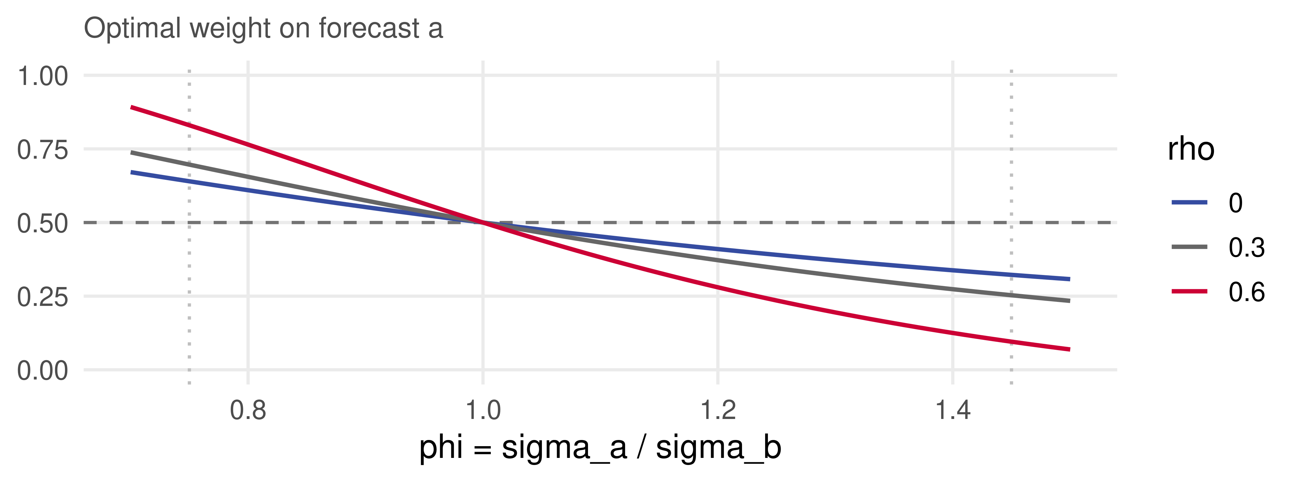
- With uncorrelated errors, error standard deviations within 30 percent of each other (\phi from 0.75 to 1.45, the dotted lines) keep \lambda^* between 0.64 and 0.32: near one half.
- Correlation spreads the weights (\rho = 0.6: from 0.83 to 0.10 over the same range), because the better forecast is also used to hedge the worse one. At \phi = 1 every curve passes through 1/2.
\lambda^* = (1 - \phi\rho) / (1 + \phi^2 - 2\phi\rho), plotted as in Diebold’s book.
And the error variance is flat around them
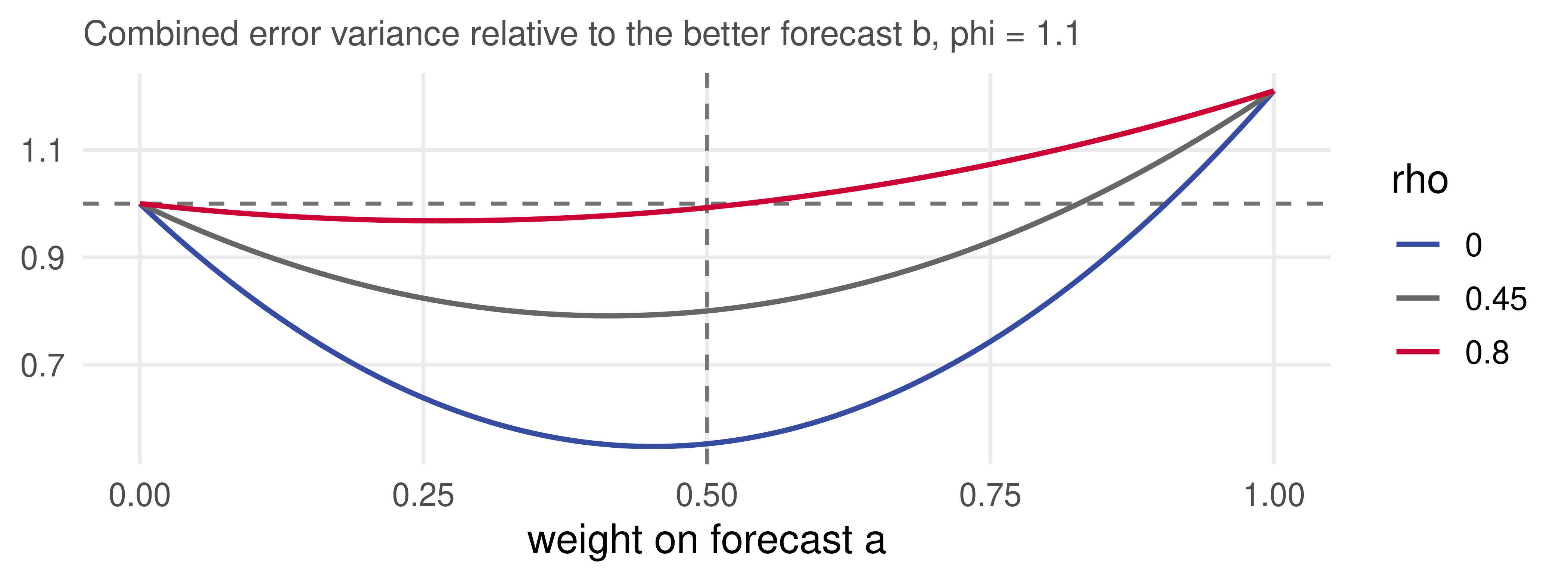
- The curves are flat near their minima. With \phi = 1.1, equal weights cost about 1 percent of the error variance when \rho is 0 or 0.45, and 2.5 percent when \rho = 0.8.
- The gain from combining at all shrinks with \rho: 45, 21 and 3 percent below the better forecast. Almost all of the gain comes from combining; almost none from the exact weight.
After a figure in Diebold’s book, which normalizes by \sigma_a^2 instead. Relative variance \lambda^2\phi^2 + (1-\lambda)^2 + 2\lambda(1-\lambda)\rho\phi.
The puzzle in a simulation
Estimate the Bates-Granger weight on T past errors and evaluate it in population (\phi = 1.1, \rho = 0.5, \lambda^* = 0.41):
set.seed(354); phi <- 1.1; rho <- 0.5
S <- matrix(c(phi^2, phi * rho, phi * rho, 1), 2)              # error covariance: sd_a = 1.1, sd_b = 1
pv <- function(l) drop(c(l, 1 - l) %*% S %*% c(l, 1 - l))     # population variance of a combination
lam_star <- (1 - phi * rho) / (1 + phi^2 - 2 * phi * rho)
puzzle <- sapply(c(20, 50, 100, 400), function(T) {
  lam_hat <- replicate(2000, bg_weights(matrix(rnorm(2 * T), T) %*% chol(S))[1])
  c(T = T, sd_lambda_hat = sd(lam_hat), equal_weights = pv(0.5) / pv(lam_star),
    estimated_weights = mean(sapply(lam_hat, pv)) / pv(lam_star))
})
round(t(puzzle), 3)
## T sd_lambda_hat equal_weights estimated_weights
## [1,] 20 0.206 1.012 1.058
## [2,] 50 0.125 1.012 1.021
## [3,] 100 0.088 1.012 1.010
## [4,] 400 0.043 1.012 1.002Equal weights cost about one percent of the error variance whatever T. Estimated weights cost more than that until the error history is a hundred observations long: the puzzle is estimation error.
Population error variance relative to its minimum, averaged over 2000 draws of the estimation sample (Smith and Wallis, 2009).
Why equal weights win so often
In forecasting competitions the simple average frequently beats combinations with “optimal” estimated weights (Stock and Watson, 2004, called it the forecast combination puzzle). The pieces of the explanation:
- Estimation error. Optimal weights must be estimated from short, noisy error histories, and the forecasts are collinear. Equal weights are slightly biased but have no variance; the same bias-variance tradeoff that favors parsimonious models favors them.
- Instability. Relative accuracy drifts, so yesterday’s optimal weights are not today’s. Equal weights cannot be wrong about the drift.
- Similar accuracy. Competing forecasts usually have similar error variances, where the figure shows the optimum close to one half anyway, and the loss from imposing it is tiny.
The equal-weights constraint is extreme shrinkage. Coaxing estimated weights toward equality rather than forcing them (the shrinkage row of the table) often does best of all: the data speak when they have something to say.
Smith and Wallis (2009) and Claeskens et al. (2016) formalize the estimation-error explanation; the 1/N portfolio of DeMiguel, Garlappi and Uppal (2009) is the same finding in finance.
A conservative argument for equal weights
Suppose we know nothing about \phi and \rho and want weights that are best in the worst case: a game between the Econometrician, who picks \lambda, and Nature, who picks the error variances and correlation to make the combined variance as large as possible.
Nature’s worst case is two forecasts of equal accuracy, \phi = 1, with perfectly correlated errors, \rho = 1: then nothing can be diversified away and no weight does better than any other. Against that opponent the Econometrician’s best response is \lambda^* = 1/2, and the pair is a Nash equilibrium of the game.
The minimax argument does not resolve the puzzle, which is about quadratic loss on average, but it shows that equal weights are the right answer when you refuse to guess the error structure. When you are willing to guess, estimated weights shrunk toward equality use what the data offer.
Diebold’s minimax argument, in the spirit of Wald’s criterion.
Application: OverSea Shipping revisited
Where we left the two forecasts
Realized volume and two two-week-ahead forecasts, 499 weeks. In the evaluation lecture: the quantitative forecast was unbiased and more accurate (RMSE 1.26 against 1.48); the judgmental forecast was biased by a full unit but had the smaller error variance; both failed the Mincer-Zarnowitz test.
##  sd_q  sd_j   phi   rho
## 1.263 1.064 1.187 0.544
Both ingredients for combination are present: neither forecast is optimal, and the error correlation of 0.54 is positive but far from one. The error standard deviation ratio is \phi = 1.19, with the judgmental forecast the less dispersed of the two.
Diebold’s textbook application; data/shipping_volume.csv.
The combining regression
Regress realized volume on both forecasts, with MA(1) disturbances for the two-step overlap. This is also the encompassing test:
##              estimate  s.e.
## ma1             0.947 0.022
## intercept       2.210 0.286
## quantitative    0.292 0.038
## judgmental 0.628 0.040- Neither forecast encompasses the other: both weights are many standard errors from zero, and the intercept is large and significant, absorbing the judgmental bias.
- The judgmental forecast gets the larger weight, 0.63 against 0.29, in spite of its higher RMSE. Once its bias is corrected it is the more accurate of the two, and the weights know it.
Diebold reports the same regression. The weights sum to 0.92, not one: the regression is free to shrink the forecasts toward the intercept, the Mincer-Zarnowitz correction at work.
Variance-covariance weights, for comparison
The Bates-Granger weight on the quantitative forecast, from the sample error variances and covariance:
## lambda_q     bg_q     bg_j
##    0.317    0.317    0.683
The same answer from the formula and from the general solution: about a third of the weight on the quantitative forecast, two thirds on the judgmental one, matching the regression’s 0.29 and 0.63 up to the regression’s bias correction. The judgmental forecast’s smaller error variance is what earns it the weight.
bg_weights() solves \Sigma \lambda \propto \iota and normalizes. Demeaning the errors first does not change it: the variance-covariance method ignores bias, which is why the regression version is preferable.
An honest test: estimate, then forecast
In-sample fits flatter any combination. Estimate everything on the first 250 weeks, then evaluate on weeks 251 to 499 with the weights held fixed:
est <- 1:250; oos <- 251:499
b_q <- mean(sh$eq[est]); b_j <- mean(sh$ej[est])                  # biases in the estimation sample
w_bg <- bg_weights(cbind(sh$eq[est] - b_q, sh$ej[est] - b_j))     # BG weights from debiased errors
w_ols <- coef(lm(Volume ~ Quantitative + Judgmental, sh[est, ]))  # unrestricted combining regression
round(c(lambda_q = unname(w_bg[1]), w_ols), 2)
## lambda_q (Intercept) Quantitative Judgmental
## 0.35 2.00 0.32 0.60f <- with(sh, list(quantitative = Quantitative, judgmental = Judgmental,
judgmental_debiased = Judgmental + b_j, equal = (Quantitative + Judgmental) / 2,
equal_debiased = (Quantitative + b_q + Judgmental + b_j) / 2,
bates_granger = w_bg[1] * (Quantitative + b_q) + w_bg[2] * (Judgmental + b_j),
regression = w_ols[1] + w_ols[2] * Quantitative + w_ols[3] * Judgmental))
round(sapply(f, function(x) rmse(sh$Volume[oos] - x[oos])), 3)## quantitative judgmental judgmental_debiased equal
## 1.257 1.497 1.021 1.150
## equal_debiased bates_granger regression
## 1.002 0.973 0.992Reading the out-of-sample results
- Bias correction alone cuts the judgmental RMSE from 1.50 to 1.02: the biased loser becomes the best single forecast. The Mincer-Zarnowitz lesson of the evaluation lecture, in money.
- Equal weights on the raw forecasts help (1.15) because the two biases partly offset; equal weights on the debiased forecasts do better still (1.00).
- Estimated weights gain a little more: 0.97 for Bates-Granger, 0.99 for the unrestricted regression, against 1.26 for the quantitative forecast that won the evaluation lecture’s horse race. A 23 percent reduction in RMSE from information the firm already had.
The ranking is the textbook one: fix the bias, then combine, and expect estimated weights to add only a little over equal ones. Note also what the regression bought relative to Bates-Granger: nothing, out of sample. Its extra freedom was spent on noise.
Everything, biases included, is estimated on weeks 1 to 250 only; the evaluation weeks never inform the weights.
Application: GDP growth, a model and the professionals
Two very different forecasters
In the evaluation lecture the recursive AR(2) and the median of the Survey of Professional Forecasters tied on next-quarter GDP growth, 1985 to 2019. One uses two numbers; the other uses everything forty economists know.
g <- read.csv("data/hw2_gdp_spread.csv") |> mutate(Quarter = yearquarter(quarter)); y <- g$gdp_growth
first <- which(g$Quarter == yearquarter("1984 Q4")); last <- which(g$Quarter == yearquarter("2019 Q4"))
origins <- first:(last - 1)                                        # origins; targets 1985Q1 to 2019Q4
ar2 <- sapply(origins, function(T) {                               # recursive AR(2) one-step forecasts
  yi <- y[1:T]; b <- coef(lm(yi[-(1:2)] ~ yi[2:(T - 1)] + yi[1:(T - 2)]))
  b[1] + b[2] * yi[T] + b[3] * yi[T - 1] })
spf <- read.csv("data/spf_median_rgdp_growth.csv") |>
  transmute(Quarter = yearquarter(paste(YEAR, QUARTER, sep = " Q")) + 1, spf = DRGDP3)
ev <- tibble(Quarter = g$Quarter[origins + 1], actual = y[origins + 1], ar2 = ar2) |>
  left_join(spf, by = "Quarter") |> mutate(e_ar2 = actual - ar2, e_spf = actual - spf)
round(c(RMSE_ar2 = rmse(ev$e_ar2), RMSE_spf = rmse(ev$e_spf), rho = cor(ev$e_ar2, ev$e_spf)), 3)
## RMSE_ar2 RMSE_spf rho
## 2.082 2.066 0.932A tie in accuracy, but with an error correlation of 0.93: the professionals and the autoregression are surprised by the same quarters. The diversification motive is weak from the start.
Does either encompass the other?
##             Estimate Std. Error t value
## (Intercept)   -1.064      0.857  -1.242
## spf            0.541      0.270   2.004
## ar2            0.775      0.254   3.054
Formally, neither does: both coefficients are significant, so each forecast carries information the other lacks. But look at the shape of the fit: the weights sum to 1.3 and the intercept is -1.1. The regression is partly correcting a common over-prediction (both forecasts ran high in this sample) rather than diversifying between two different views.
One-step forecasts, so ordinary HAC standard errors with no overlap correction. R^2 of the encompassing regression: 0.20.
Out of sample, again
Estimate weights on the first half of the evaluation sample (1985 to 2002) and evaluate on the second (2002 to 2019):
h1 <- 1:70; h2 <- 71:140                                           # 1985Q1-2002Q2 and 2002Q3-2019Q4
w_bg <- bg_weights(cbind(ev$e_spf[h1], ev$e_ar2[h1]))              # weights from the first half only
w_ols <- coef(lm(actual ~ spf + ar2, ev[h1, ]))
f <- with(ev, list(spf = spf, ar2 = ar2, equal = (spf + ar2) / 2,
                   bates_granger = w_bg[1] * spf + w_bg[2] * ar2,
                   regression = w_ols[1] + w_ols[2] * spf + w_ols[3] * ar2))
round(c(sapply(f, function(x) rmse(ev$actual[h2] - x[h2])), lambda_spf = unname(w_bg[1])), 3)
## spf ar2 equal bates_granger regression
## 2.024 2.204 2.097 2.133 2.128
## lambda_spf
## 0.315- In the second half the professionals pulled ahead of the AR(2): 2.02 against 2.20. Equal weights land in between (2.10); the estimated weights, learned on a first half in which the AR(2) did better, do slightly worse.
- No combination beats the better forecast: with \rho = 0.93 there is almost nothing to diversify. The combination’s virtue is insurance: whichever forecaster turns out better, the average is never far behind.
The first-half weight on the SPF is 0.3; the second half would have wanted more. Combination needs forecasts that err differently.
Survey-based combination and the wisdom of crowds
Surveys are combination machines
Several institutions regularly survey forecasters and publish consensus forecasts, the mean or median across respondents: an equal-weight combination of a few dozen information sets.
| Survey | Who | Since | What |
|---|---|---|---|
| Survey of Professional Forecasters | Philadelphia Fed (earlier ASA/NBER) | 1968 | US macro, point and density forecasts, quarterly |
| ECB Survey of Professional Forecasters | European Central Bank | 1999 | euro area macro; about 120 panelists |
| Livingston Survey | Philadelphia Fed | 1946 | US macro, twice a year |
| Blue Chip Economic Indicators | private | 1976 | monthly business-economist consensus |
| Michigan Survey of Consumers | University of Michigan | 1946 | household expectations and sentiment |
The median is robust to outliers; otherwise the consensus is the simple average of the previous section, and it performs very well relative to the individual forecasters, as we are about to see.
The SPF also collects probability distributions, from which combined density forecasts can be built.
The wisdom of crowds
Galton (1907) found the median of 787 guesses at the weight of an ox within one percent of the truth, better than any butcher present. Surowiecki (2004) made it a book. The conditions, which are the conditions for combination gains:
- Diverse, imperfectly dependent judgments, so that there is something to average out. A crowd of forecasters who all read the same model is one forecaster (\rho \to 1).
- A dispassionate aggregation mechanism that avoids groupthink. Surveys are good at this: respondents do not see each other’s answers before submitting.
Methods that violate the second condition are suspect. The Delphi method surveys experts, reveals the distribution of answers, and iterates; opinions converge, but partly through social pressure. Focus groups are worse, because a few voices dominate. Both may still be useful where nothing can be quantified, such as forecasting a technology that does not yet exist.
Other dispassionate aggregators: prices in markets, Google’s PageRank, open-source code review.
The SPF panel: individual forecasts and the consensus
Individual next-quarter GDP growth forecasts from the SPF, targets 1985 to 2019, and three consensus measures:
ind <- read.csv("data/spf_individual_rgdp_growth.csv") |>
  transmute(Quarter = yearquarter(paste(YEAR, QUARTER, sep = " Q")) + 1, ID, f = g_next) |>
  inner_join(g |> select(Quarter, actual = gdp_growth), by = "Quarter") |>
  filter(year(Quarter) >= 1985, year(Quarter) <= 2019)
cons <- ind |> group_by(Quarter, actual) |>
  summarise(n = n(), c_mean = mean(f), c_median = median(f), c_trim = mean(f, trim = 0.1),
            .groups = "drop")
round(c(forecasters = n_distinct(ind$ID), surveys = nrow(cons), responses_per_survey = mean(cons$n),
        RMSE_mean = rmse(cons$actual - cons$c_mean), RMSE_median = rmse(cons$actual - cons$c_median),
        RMSE_trimmed = rmse(cons$actual - cons$c_trim)), 3)
## forecasters surveys responses_per_survey
## 222.000 140.000 35.679
## RMSE_mean RMSE_median RMSE_trimmed
## 2.068 2.060 2.053A time series of cross sections, not a panel: forecasters join and leave (the median one answered 12 surveys), so the consensus combines a changing set of information sets. Mean, median and trimmed mean are within 0.02 of each other.
data/spf_individual_rgdp_growth.csv: growth implied by each respondent’s level forecasts; latest-vintage realizations.
Forecasters against their consensus
For each forecaster with at least 20 responses, compare their RMSE with the RMSE of the survey median over the same quarters, so that nobody is penalized for having forecast the hard years:
each <- ind |> left_join(cons |> select(Quarter, c_median), by = "Quarter") |> group_by(ID) |>
  summarise(n = n(), ratio = rmse(actual - f) / rmse(actual - c_median)) |> filter(n >= 20)
round(c(forecasters = nrow(each), share_beaten_by_median = mean(each$ratio > 1),
        quantile(each$ratio, c(0, 0.25, 0.5, 0.75, 1))), 2)
## forecasters share_beaten_by_median 0%
## 78.00 0.82 0.83
## 25% 50% 75%
## 1.02 1.06 1.10
## 100%
## 1.66The consensus median beats four forecasters in five. The median forecaster’s RMSE is 6 percent above the consensus, the worst 66 percent above it; the few who beat it did so by at most 17 percent, and nothing tells us in advance who they will be. The average of many is better than almost every one of the many.
Reading the panel
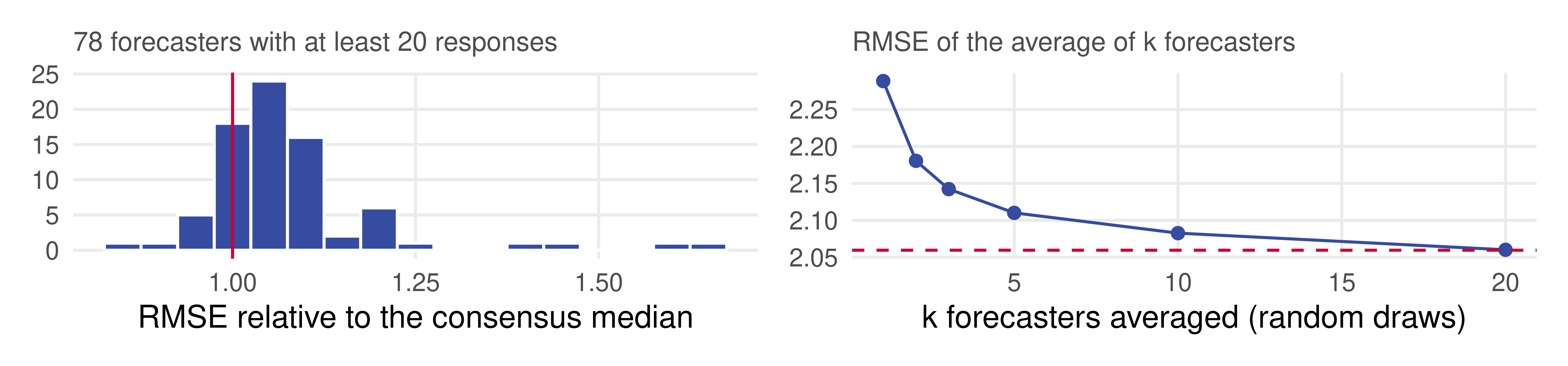
- Left. The distribution of relative RMSEs sits almost entirely to the right of one. Its left tail is short: nobody beats the consensus by much.
- Right. Averaging randomly chosen forecasters helps quickly and then flattens: two recover half of the gain from one forecaster to the full consensus, five recover three quarters. The dashed line is the full-panel median. Diversification with diminishing returns, exactly as in a portfolio.
Averages over 100 random draws of k forecasters per survey. One forecaster: RMSE 2.29, 11 percent above the consensus median.
Dispersion is not uncertainty
The spread of point forecasts across respondents is a tempting measure of how uncertain the outlook is. It is not one. Cross-sectional disagreement and the uncertainty each forecaster feels are different objects, and in principle unrelated.
##     mean_dispersion corr_with_abs_error
##               0.909               0.067
In this panel the correlation between disagreement and the size of the consensus error is essentially zero. A density forecast of GDP growth cannot be read off the histogram of point forecasts; it needs each forecaster’s own probability distribution, which the SPF also collects, and a combination of those.
Zarnowitz and Lambros (1987) made the distinction; the SPF’s probability bins are the standard source for survey-based density forecasts.
Markets as combiners
A price is also a combination: it aggregates the information of everyone who trades, weighted by how much they are willing to bet. Breakeven inflation from indexed bonds, fed funds futures, and prediction markets on elections are all forecasts of this kind, and they can be evaluated like any other.
- Markets satisfy the aggregation condition of the wisdom of crowds unusually well: dispassionate, continuous, and expensive to manipulate.
- They fail the independence condition in a particular way: traders watch each other, and bubbles are the crowd agreeing with itself. The explosive-root tests of the unit-root lecture are one way to tell.
- Market forecasts embed risk premia, so they can be biased as forecasts while being correct as prices; the Mincer-Zarnowitz regression is the right check.
Diebold’s book has a chapter on market-based combination, which this course does not cover in detail. Arrow et al. (2008) make the case for prediction markets.
What to take away
- Encompassing. If neither forecast is redundant in a regression of the realization on both, combining can help. Combination is what we do when information sets cannot be pooled in time.
- Weights. Variance-covariance weights, \lambda^* = (\sigma_b^2 - \sigma_{ab}) / (\sigma_a^2 + \sigma_b^2 - 2\sigma_{ab}), are the minimum-variance portfolio of forecasts and a special case of the combining regression, which also corrects bias. Nothing to lose in population; estimation error and instability to lose in samples.
- Equal weights are hard to beat because the optimum is usually near one half and has to be estimated from noisy, collinear data. Shrink toward them rather than force them.
- Applications. OverSea: debias, then combine, for a 23 percent RMSE reduction. GDP: a model and the professionals erred together (\rho = 0.93), so combination insured rather than improved.
- Surveys are equal-weight combinations of dozens of information sets; the SPF median beats four forecasters in five. Disagreement among them is not a measure of uncertainty.
R cheat sheet
library(fpp3); library(sandwich); library(lmtest)
# ---- encompassing and combining regressions ---------------------------------------------
lm(y ~ f_a + f_b); hac_table(lm(y ~ f_a + f_b), lag = h - 1)      # unrestricted combination; HAC table (these slides)
arima(y, order = c(0, 0, h - 1), xreg = cbind(f_a, f_b))         # the same with MA(h-1) disturbances
# ---- variance-covariance weights ----------------------------------------------------------
S <- cov(cbind(e_a, e_b)); (S[2, 2] - S[1, 2]) / (S[1, 1] + S[2, 2] - 2 * S[1, 2])   # two forecasts
bg_weights(E)                     # N forecasts: solve(cov(E), 1), normalized (these slides)
# ---- out-of-sample protocol ---------------------------------------------------------------
w <- bg_weights(E[est, ]); fc <- F[ev, ] %*% w; rmse(y[ev] - fc)  # estimate weights on est, evaluate on ev
# ---- surveys ------------------------------------------------------------------------------
ind |> group_by(Quarter) |> summarise(median(f), mean(f, trim = 0.1))   # consensus from individual responses
# packages: ForecastComb (comb_BG, comb_OLS, comb_SA, comb_LAD, ...) implements the classic schemes
References
Additional resources
- Textbooks
- Diebold, F.X. Forecasting in Economics, Business, Finance and Beyond, the chapters on model-based, market-based and survey-based forecast combination. Timmermann, A. (2006), “Forecast Combinations,” in Handbook of Economic Forecasting, Vol. 1, Elsevier, for a thorough survey.
- Original sources
- Bates, J.M. and Granger, C.W.J. (1969), “The Combination of Forecasts,” Operational Research Quarterly, 20, 451–468. Granger, C.W.J. and Ramanathan, R. (1984), “Improved Methods of Combining Forecasts,” Journal of Forecasting, 3, 197–204.
- Chong, Y.Y. and Hendry, D.F. (1986), Review of Economic Studies, 53, 671–690; Fair, R.C. and Shiller, R.J. (1990), American Economic Review, 80, 375–389. Clemen, R.T. (1989), “Combining Forecasts: A Review and Annotated Bibliography,” International Journal of Forecasting, 5, 559–583.
Additional resources (continued)
- Original sources (continued)
- Stock, J.H. and Watson, M.W. (2004), “Combination Forecasts of Output Growth in a Seven-Country Data Set,” Journal of Forecasting, 23, 405–430. Smith, J. and Wallis, K.F. (2009), Oxford Bulletin of Economics and Statistics, 71, 331–355. Claeskens, G., Magnus, J.R., Vasnev, A.L. and Wang, W. (2016), International Journal of Forecasting, 32, 754–762.
- Diebold, F.X. and Shin, M. (2019), “Machine Learning for Regularized Survey Forecast Combination: Partially-Egalitarian LASSO and its Derivatives,” International Journal of Forecasting, 35, 1679–1691. Shi, Z., Su, L. and Xie, T. (2022), “\ell_2-Relaxation: With Applications to Forecast Combination and Portfolio Analysis,” Review of Economics and Statistics (code: L2Relax, LasForecast). DeMiguel, V., Garlappi, L. and Uppal, R. (2009), Review of Financial Studies, 22, 1915–1953.
- Surowiecki, J. (2004), The Wisdom of Crowds, Doubleday. Galton, F. (1907), “Vox Populi,” Nature, 75, 450–451. Zarnowitz, V. and Lambros, L.A. (1987), Journal of Political Economy, 95, 591–621.
- Data:
data/shipping_volume.csv;data/hw2_gdp_spread.csv;data/spf_median_rgdp_growth.csvanddata/spf_individual_rgdp_growth.csv(Survey of Professional Forecasters, Federal Reserve Bank of Philadelphia, downloaded October 2026).