By now we can produce forecasts from trends, seasonals, autoregressions, GARCH models, VARs, and from no model at all. Each application ended with a plot of forecast against realization and a number or two. That is not evaluation.
Two questions make it evaluation. Absolute: does a forecast have the properties an optimal forecast must have, so that no cheap fix would improve it? Relative: is one forecast more accurate than another, and is the difference more than luck?
Today: the unforecastability principle and the tests it implies; accuracy measures, benchmarks and forecastability; the Diebold-Mariano test; two applications, a shipping company’s forecasts and quarterly GDP growth; and how to evaluate interval and density forecasts, with the volatility models of a few weeks ago as the test case.
Diebold, Forecasting in Economics, Business, Finance and Beyond, the chapters on evaluating point forecasts and on evaluating interval and density forecasts. The shipping data come from the book’s companion files; the professional forecasts from the Survey of Professional Forecasters.
Absolute standards: the unforecastability principle
What an optimal forecast looks like
For a covariance stationary series with Wold representation y_t = \mu + \varepsilon_t + b_1 \varepsilon_{t-1} + b_2 \varepsilon_{t-2} + \cdots, the h-step linear least squares forecast and its error are
The error is made entirely of shocks that arrive after the forecast is made. Hence the one property from which all others follow, the unforecastability principle:
Optimal forecast errors are unforecastable from information available when the forecast was made.
It holds in great generality: for conditional-mean or linear-projection optimality, for any loss function, and for nonstationary series too. If you could forecast the error, you could add that forecast to the forecast and do better; so an optimal forecast leaves nothing forecastable behind.
Four properties that follow
Optimal forecasts are unbiased: E(e_{t+h,t}) = 0.
Optimal one-step errors are white noise: e_{t+1,t} = \varepsilon_{t+1}.
Optimal h-step errors are at most MA(h-1): h - 1 future shocks overlap between e_{t+h,t} and e_{t+h+1,t+1}, so autocorrelations up to displacement h-1 may be nonzero, and those beyond must be zero.
Optimal h-step error variances are nondecreasing in h and converge to the unconditional variance of the series.
Each is a testable restriction on a series we observe: the forecast errors. The tests that follow are all applications of the same idea, with one wrinkle: for h > 1 the errors are serially correlated even when the forecast is perfect, so standard errors must allow for it.
Property (c) is what made the multi-step errors in the ARMA forecasting lecture an MA(h-1).
Testing optimality: bias, white noise, orthogonality
Are the errors zero-mean?
Regress the forecast errors on a constant and test whether the mean is zero.
If e_{t+h,t} is Gaussian white noise, as one-step errors might be, the ordinary t statistic does the job; iid but non-Gaussian errors need only large samples.
For h > 1 the errors are serially correlated even under optimality, and they may be serially correlated because the forecast is not optimal. Either way the disturbance of the regression on a constant must be modeled: start with MA(h-1) disturbances, let AIC and SIC say whether more is needed, or use heteroskedasticity and autocorrelation consistent (HAC, Newey-West) standard errors.
In R, arima(e, order = c(0, 0, h - 1)) estimates the mean with MA(h-1) disturbances and reports its standard error; sandwich::NeweyWest() gives the HAC alternative. These slides use a helper, hac_t(e, lag = h - 1), that returns the HAC t statistic of the mean.
“Bias” is a population statement, so even a clearly nonzero sample mean error needs a standard error before it becomes a verdict.
White noise, and at most MA(h−1)
One-step errors. The correlogram with its \pm 2/\sqrt{T} bands, and the Ljung-Box Q statistics, exactly as for residuals in the cycles lectures. The Durbin-Watson statistic is a weaker check that looks at the first autocorrelation only.
h-step errors. The MA(h-1) structure means a cutoff: autocorrelations beyond displacement h - 1 should be inside the bands. For a formal test, regress the errors on a constant with MA(q) disturbances, q > h - 1, and test whether the moving-average coefficients beyond h - 1 are zero.
Variances. Plot the sample h-step error variance against h. It should rise and flatten; its pattern tells how fast the forecast’s information decays.
Serial correlation in one-step errors is the most common symptom of a fixable forecast: the error was forecastable from its own past, so a model of the errors would have improved the forecast.
Orthogonality and the Mincer-Zarnowitz regression
The tests so far use only the errors’ own past. The principle says more: errors should be orthogonal to anything in the information set. Regress them on candidate variables and test that all slopes are zero:
The most important candidate is the forecast itself, which is certainly in the information set. Equivalently, regress the realization on the forecast, the Mincer-Zarnowitz regression:
Subtracting y_{t+h,t} from both sides shows the two regressions are the same test: (\beta_0, \beta_1) = (0, 1) is (\alpha_0, \alpha_1) = (0, 0).
\beta_0 \neq 0 is bias; \beta_1 < 1 says the forecast over-reacts to its own information and should be shrunk toward the mean. Rejection is constructive: the fitted regression is itself an improved forecast. The Wald test of the joint hypothesis uses HAC standard errors when h > 1.
Mincer and Zarnowitz (1969). mz_test(y, f, lag = h - 1) in these slides reports the coefficients and the Wald test.
Ranking forecasts needs a loss function L(e) (recall the loss-function lecture) and a horizon. With errors e_{t+h,t} = y_{t+h} - y_{t+h,t} over t = 1, \ldots, T:
MSE = \text{variance} + \text{bias}^2 is the bias-variance tradeoff: under quadratic loss a biased forecast can beat an unbiased one with more dispersed errors. A small bias for a large variance reduction is a good trade.
MSE squares the units; RMSE and MAE keep them. MAE is less sensitive to a few huge errors.
Benchmarks: predictive R² and Theil’s U
Accuracy numbers mean little in isolation. Compare them with an allegedly naive benchmark:
Predictive R^2 replaces the in-sample residuals of the usual R^2 by out-of-sample one-step errors, so it compares the forecast with the historical mean forecast \bar y. Near 1 is good; near 0 says the model forecasts no better than the mean; negative is worse.
Theil’s U changes the benchmark to the no-change forecast y_{t-1}. Meteorologists call such numbers skill scores. The h-step versions replace e_{t,t-1} by e_{t,t-h}.
Naive benchmarks are not always naive. Many economic series are nearly random walks, and then no forecaster beats “no change” by much, through no fault of their own: the yen of the unit-root lecture. A skill score near zero may be the honest ceiling.
Theil (1966). Both benchmarks must be computed out of sample too: an expanding-window mean, and the last observation.
How forecastable is a series?
Even an optimal forecast makes errors; how large they are is a property of the series. Under quadratic loss, patterned after R^2,
G = 1 - \frac{\operatorname{var}(e_{t+j,t})}{\operatorname{var}(y_{t+j})}, \qquad\text{and more generally}\qquad
P(L, \Omega, j, k) = 1 - \frac{E\,L(e_{t+j,t})}{E\,L(e_{t+k,t})}, \quad j \ll k :
the expected loss of an optimal short-horizon forecast relative to that of a long-horizon one. G is the special case of quadratic loss and k = \infty.
Predictability is a matter of degree, and it depends on the horizon, the loss and the information set. P accommodates all three, and difference-stationary series as well (keep k finite).
A random walk has P = 1 - j/k: forecastable at short horizons relative to long ones, yet its persistence (the variance ratio j) is a different concept. White noise has P = 0.
Volatility is not predictability either: predictability is the ratio of conditional to unconditional variance, volatility the unconditional variance alone.
Diebold and Kilian (2001). In practice P is estimated from a fitted model’s forecast error variances.
Forecastability by horizon: Canadian employment
The AR(2) of the cycles lectures, \hat\phi_1 = 1.44, \hat\phi_2 = -0.48, implies \sigma_h^2 = \sigma^2 \sum_{i<h} \psi_i^2 and \operatorname{var}(y) = \sigma^2 \sum_i \psi_i^2, hence P(h) = G at each horizon:
Employment is 96 percent forecastable one quarter ahead, two thirds a year ahead, and 4 percent five years ahead. The same calculation for quarterly GDP growth gives about 0.1 at h = 1: GDP growth is nearly unforecastable from its own past, which sets the bar for the application below.
Is the difference real? The Diebold-Mariano test
Horse races
Two forecasts of US inflation: the Survey of Professional Forecasters (S) and the breakeven rate from inflation-indexed bonds (B). Over some sample, \widehat{MSE}_S = 1.80 and \widehat{MSE}_B = 1.92. “S wins.”
Does it? Even if the two population MSEs were identical, one of the two sample MSEs would be smaller. The question in any sample is whether S is truly superior or merely lucky. That is a hypothesis test, with the hypothesis of equal predictive accuracy
The population statement is about expected loss; we test it with the sample average of the loss differentiald_t, a constructed but observed series.
The forecasts may come from models, surveys, markets or judgment: the test treats the forecast errors as primitives and never asks where they came from.
The Diebold-Mariano test
Assume only that the loss differential is covariance stationary:
where \hat\sigma_{\bar d} is a consistent estimate of the standard deviation of the sample mean, which must allow for serial correlation in d_t: forecast errors overlap when h > 1, and suboptimal forecasts have serially correlated errors at any horizon.
That is all: one assumption, one statistic, one limiting distribution. DM is a t test that the mean of d_t is zero, with the standard error computed robustly. Regress d_t on a constant with HAC standard errors, or with MA(h-1) or AR(p) disturbances chosen by AIC.
Diebold and Mariano (1995). Covariance stationarity is sufficient, not necessary; mixing conditions would do.
Reading Assumption DM
All models are false, but some are useful (Box). No loss differential is exactly stationary, just as no economic series is; the question is whether stationarity is a useful approximation.
Forecasters aim at it. Optimal forecasts have unforecastable, covariance stationary errors, hence stationary loss differentials. Suboptimal forecasts have serially correlated errors, which HAC standard errors absorb; a unit root in the errors would be serial correlation taken to the extreme.
Nonstationarities tend to cancel. Forecasters share information, so a common nonstationary loss component drops out of the difference: L(e_{at}) = x_t + \eta_{at} and L(e_{bt}) = x_t + \eta_{bt} give a stationary d_t even if neither loss is stationary.
It is testable. Plot d_t, look at its correlogram, test it for unit roots and breaks.
Extensions. The regression form invites conditioning: add variables that may explain the loss differential, such as a recession indicator, to ask when one forecast is better (Giacomini and White, 2006). The loss need not be quadratic: |e|, direction-of-change, anything.
Diebold (2015) revisits the test twenty years on. Comparing nested models estimated on the same data changes the limit distribution (West, 1996; Clark and McCracken, 2001); treating forecasts as primitives sidesteps this.
Application: OverSea Shipping
Two forecasts of shipping volume
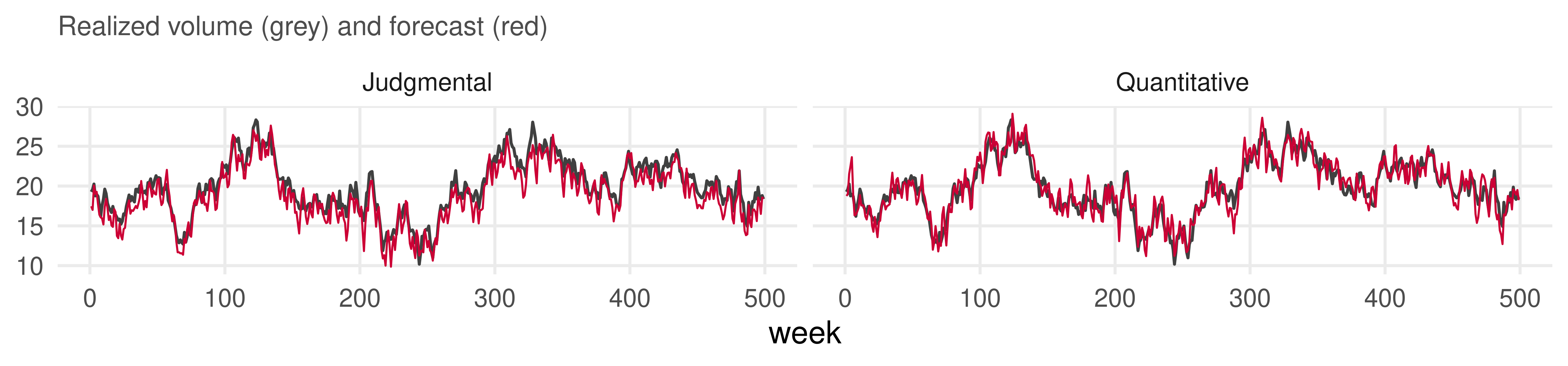
OverSea Services ships cargo across the Atlantic and forecasts weekly volume on each trade lane twice: a quantitative forecast from a model and a judgmental forecast from its sales representatives. Here: the North America to Europe lane, realized volume and the two two-week-ahead forecasts, 499 weeks.
sh <-read.csv("data/shipping_volume.csv") # Week, Volume, Judgmental, Quantitative
Both forecasts track the realization closely: two weeks ahead is not far. The differences are in the details.
data/shipping_volume.csv, January 1988 to July 1997: Diebold’s textbook application, data from its companion files.
The forecast errors
sh <- sh |>mutate(eq = Volume - Quantitative, ej = Volume - Judgmental) # realization minus forecast
stats <-function(e) { z <- (e -mean(e)) /sd(e)c(mean =mean(e), sd =sd(e), RMSE =sqrt(mean(e^2)), MAE =mean(abs(e)),skewness =mean(z^3), kurtosis =mean(z^4)) }round(rbind(quantitative =stats(sh$eq), judgmental =stats(sh$ej)), 3)
Quantitative errors are centered on zero; judgmental errors sit about one unit above it (realized volume ran higher than the sales force predicted, a pessimistic bias) but are less dispersed. Both look normal.
Error correlograms
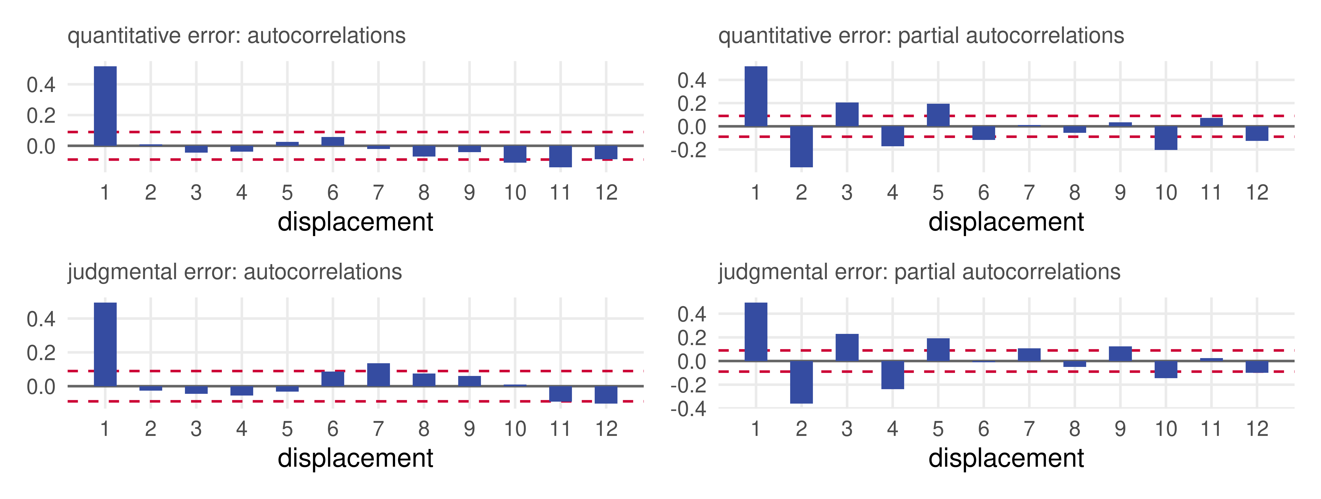
In both cases the autocorrelations cut off after displacement 1 (0.52 and 0.50) and the partial autocorrelations oscillate and decay: the MA(1) structure that optimal two-step-ahead errors should have. Property (c) passes.
Is either forecast biased?
Two-step errors are MA(1), so regress each error series on a constant with MA(1) disturbances and read off the t statistic of the mean:
bias <-function(e) { m <-arima(e, order =c(0, 0, 1)) # mean with MA(1) disturbances mu <-coef(m)["intercept"]; se <-sqrt(m$var.coef["intercept", "intercept"])round(c(mean =unname(mu), s.e. = se, t =unname(mu / se), theta =unname(coef(m)["ma1"])), 3)}rbind(quantitative =bias(sh$eq), judgmental =bias(sh$ej))
##                mean  s.e.      t theta
## quantitative -0.027 0.080 -0.333 0.934
## judgmental    1.023 0.067 15.261 0.960
c(HAC_t_quantitative =hac_t(sh$eq, lag =1), HAC_t_judgmental =hac_t(sh$ej, lag =1))
No bias in the quantitative forecast. A bias of one unit in the judgmental forecast, with a t statistic of 15: sizable and overwhelmingly significant. The HAC version agrees.
Ignoring the MA(1) term would badly understate the standard error of the mean; Diebold reports the same estimates.
Mincer-Zarnowitz regressions
Regress realized volume on each forecast, with HAC standard errors for the two-step overlap, and test (\beta_0, \beta_1) = (0, 1):
rbind(quantitative =mz_test(sh$Volume, sh$Quantitative, lag =1),judgmental =mz_test(sh$Volume, sh$Judgmental, lag =1))
Both fail, decisively. We expected the judgmental forecast to fail, because it is biased. But until now the quantitative forecast had passed every check; the MZ regression finds a slope well below one: the forecast over-reacts to its own information, and shrinking it toward the mean, 2.2 + 0.89\, \hat y, would have been better. Rejection is constructive.
Diebold runs the same regressions with MA(1) disturbances instead of HAC standard errors; same verdict. The orthogonality tests use only information available at forecast time, so the improvement was feasible.
Which is more accurate?
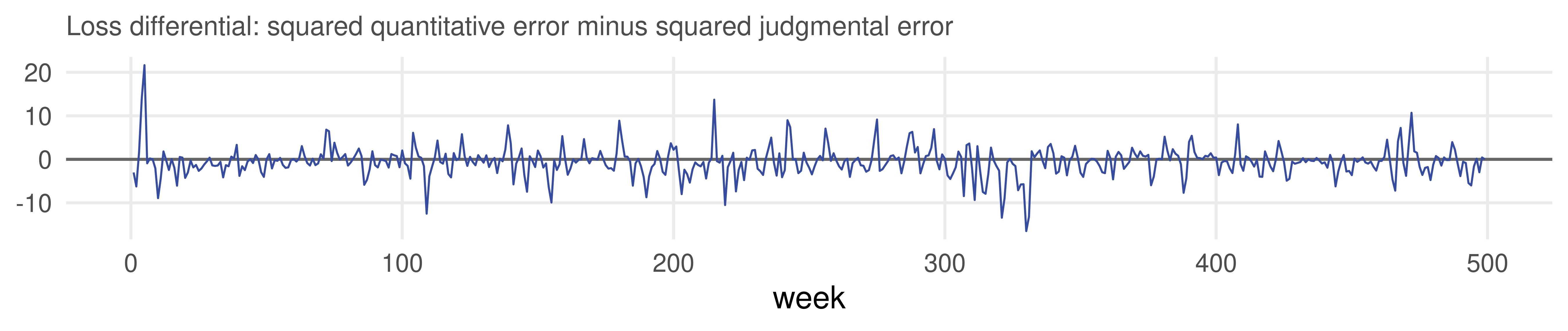
Under quadratic loss the quantitative forecast wins: RMSE 1.26 against 1.48 (MAE 1.00 against 1.23). The judgmental errors are less dispersed, so the whole gap is the bias. Is the gap real? Form the loss differential:
sh <- sh |>mutate(d = eq^2- ej^2) # quadratic loss differentialround(c(mean =mean(sh$d), sd =sd(sh$d), acf =acf(sh$d, 3, plot =FALSE)$acf[-1]), 3)
The mean, -0.58, is small relative to the standard deviation, 3.4, but the 499 observations and the MA(1) serial correlation (\hat\rho(1) = 0.36, then nothing) are what the test must account for.
The Diebold-Mariano test, three ways
dm_ma1 <-arima(sh$d, order =c(0, 0, 1)) # mean with MA(1) disturbancesc(DM_MA1 =unname(coef(dm_ma1)["intercept"] /sqrt(dm_ma1$var.coef["intercept", "intercept"])),DM_HAC =hac_t(sh$d, lag =1))
##    DM_MA1    DM_HAC
## -2.865698 -3.286535
forecast::dm.test(sh$eq, sh$ej, h =2, power =2)$statistic # the packaged version
##        DM
## -2.915281
All three put DM near -3, with a p-value below 0.01. The quantitative forecast is more accurate under quadratic loss, and the verdict is not luck. Under absolute loss (power = 1) the statistic is -3.5.
And yet the loser has the smaller error variance. A bias-corrected judgmental forecast would be a serious competitor, and the two together might beat either. That is next week’s subject.
dm.test() uses a rectangular-window variance estimate with h - 1 autocovariances; the Newey-West version uses Bartlett weights; the MA(1) version models the dependence parametrically. They agree because the loss differential really is MA(1).
Application: GDP growth
Six forecasts of next quarter’s growth
Quarterly real GDP growth (annualized percent) and the term spread from the second homework. Recursive one-quarter-ahead forecasts: at each origin T from 1984Q4, estimate on 1959 to T and forecast T + 1; 140 forecasts, 1985Q1 to 2019Q4.
g <-read.csv("data/hw2_gdp_spread.csv") |>mutate(Quarter =yearquarter(quarter))y <- g$gdp_growth; s <- g$spreadorigins <-which(g$Quarter ==yearquarter("1984 Q4")):(which(g$Quarter ==yearquarter("2019 Q4")) -1)fc <-t(sapply(origins, function(T) { # one row of forecasts per origin T yi <- y[1:T]; si <- s[1:T] d <-data.frame(y = yi[-(1:2)], l1 = yi[2:(T -1)], l2 = yi[1:(T -2)], sp = si[2:(T -1)]) nd <-data.frame(l1 = yi[T], l2 = yi[T -1], sp = si[T]) # the regressors for T + 1 f <-function(m) unname(predict(lm(m, d), nd))c(mean =mean(yi), nochange = yi[T], ar1 =f(y ~ l1), ar2 =f(y ~ l1 + l2),ar2_spread =f(y ~ l1 + l2 + sp))}))ev <-tibble(Quarter = g$Quarter[origins +1], actual = y[origins +1]) |>bind_cols(as_tibble(fc))
Five model forecasts: the expanding-window mean, no change, AR(1), AR(2), and the AR(2) with the lagged spread, significant in the homework. A sixth is model-free: the SPF median.
data/hw2_gdp_spread.csv. The evaluation stops in 2019: the 2020 quarters (-30 and +35 percent) would account for most of every squared-error measure.
Adding the professional forecasters
spf <-read.csv("data/spf_median_rgdp_growth.csv") |>transmute(Quarter =yearquarter(paste(YEAR, QUARTER, sep =" Q")) +1, # target: survey quarter + 1spf = DRGDP3)ev <- ev |>left_join(spf, by ="Quarter")models <-c("mean", "nochange", "ar1", "ar2", "ar2_spread", "spf")err <-as_tibble(sapply(models, function(m) ev$actual - ev[[m]])) # errors: actual minus forecastacc <-function(e) c(ME =mean(e), RMSE =sqrt(mean(e^2)), MAE =mean(abs(e)))round(t(sapply(err, acc)), 3)
The AR(2) is the most accurate model by RMSE and MAE; adding the spread makes the forecasts worse. The professionals, with every indicator at hand, match the AR(2) and are the only unbiased forecast in the table.
data/spf_median_rgdp_growth.csv: Philadelphia Fed, median forecast DRGDP3. The survey is taken mid-quarter, so its “next quarter” forecast made in quarter t targets growth in t+1. Realizations are the latest vintage; the SPF forecast the first release.
Benchmarks and absolute checks
rel <-function(e, b) 1-sum(e^2) /sum(b^2) # predictive R2 against the benchmark errors bround(c(R2_ar2 =rel(err$ar2, err$mean), R2_ar2_spread =rel(err$ar2_spread, err$mean),R2_spf =rel(err$spf, err$mean), U_ar2 =rel(err$ar2, err$nochange),U_mean =rel(err$mean, err$nochange)), 3)
Predictive R^2 of 0.20: the AR(2) removes a fifth of the error variance of the historical mean. Quarterly GDP growth is hard to forecast; the spread model keeps only 0.06.
Mincer-Zarnowitz: the AR(2) passes, narrowly; the SPF passes with a slope of 0.95; the spread model fails with a slope of 0.68: its forecasts over-react and should be shrunk.
AR(2) errors: mean -0.36 (HAC t = -2.1), no serial correlation (Q(8): p = 0.85), and t = 0.9 on the lagged spread.
Multi-step errors behave as they should
Iterate the recursive AR(2) forecasts to horizons two to four and look at the errors:
hfc <-t(sapply(origins, function(T) { # AR(2) chain-rule forecasts, h = 1, ..., 4 yi <- y[1:T]; b <-coef(lm(yi[-(1:2)] ~ yi[2:(T -1)] + yi[1:(T -2)])) path <- yi[(T -1):T]for (h in1:4) path <-c(path, b[1] + b[2] * path[length(path)] + b[3] * path[length(path) -1]) path[-(1:2)]}))t(sapply(1:4, function(h) { # errors at each horizon, within the sample ok <- origins + h <=max(origins) +1; e <- y[origins[ok] + h] - hfc[ok, h]round(c(h = h, RMSE =sqrt(mean(e^2)), acf =acf(e, 3, plot =FALSE)$acf[-1]), 3)}))
The RMSE rises with the horizon and flattens quickly near the standard deviation of growth (2.25), property (d); the error autocorrelations grow with h as an MA(h-1) allows, property (c). A series this unpredictable reaches its unconditional variance within a year.
Is the AR(2) really better? Diebold-Mariano
dm <-function(a, b) hac_t(err[[a]]^2- err[[b]]^2, lag =0) # negative favors the first forecastround(c(`AR(2) vs mean`=dm("ar2", "mean"), `AR(2) vs no change`=dm("ar2", "nochange"),`AR(2) vs AR(2)+spread`=dm("ar2", "ar2_spread"), `AR(2) vs AR(1)`=dm("ar2", "ar1"),`SPF vs AR(2)`=dm("spf", "ar2"), `SPF vs mean`=dm("spf", "mean")), 2)
##         AR(2) vs mean    AR(2) vs no change AR(2) vs AR(2)+spread
##                 -2.41                 -2.65                 -2.80
##        AR(2) vs AR(1)          SPF vs AR(2)           SPF vs mean
##                 -2.22                 -0.18                 -1.70
The AR(2) beats the mean, no change, the AR(1) and the spread model at the 5% level or better. The spread’s in-sample t statistic of 2.5 over 1959 to 2019 did not survive out of sample: the parsimony lesson of the forecasting-basics lecture, now with a test attached.
The SPF and the AR(2) are statistically indistinguishable one quarter ahead (DM = -0.2), and the SPF’s edge over the mean is marginal (-1.7).
One-step errors, so lag = 0; a Newey-West lag of 4 changes nothing. Under absolute loss the AR(2)-versus-spread statistic is -1.8: the spread model’s extra errors are a few large ones.
Interval and density forecast evaluation
Correct on average, or correct at every date?
A (1-\alpha) interval forecast is unconditionally calibrated if it brackets the realization (1-\alpha) of the time in the long run. It is conditionally calibrated if it does so at every date, given what was known then.
The volatility lecture made the distinction concrete. Constant-width intervals in a GARCH world can be right on average and wrong at almost every date: too wide in calm periods, too narrow in turbulent ones, with misses clustered in the turbulent ones. The 70-day comparison there was suggestive; a proper evaluation needs a long sequence and a test.
Define the hit sequence of a one-step interval forecast,
I_t = \mathbf{1}\{ y_t \text{ falls inside the interval forecast made at } t-1 \}.
Under correct conditional calibration, I_t \sim \text{iid Bernoulli}(1 - \alpha): the right mean and independence. The hit sequence is the interval forecast’s “error”, and like every one-step error it should be unforecastable.
Christoffersen (1998). For h-step intervals the hits need not be independent but should have (h-1)-dependent structure.
Christoffersen’s tests
Two likelihood-ratio tests separate the two parts of the hypothesis. With n_1 hits and n_0 misses, and \hat\pi = n_1 / (n_0 + n_1),
tests unconditional coverage. For independence, fit a first-order Markov chain to the hit sequence and test whether the probability of a hit depends on whether the last period was a hit:
with n_{ij} the number of transitions from state i to state j and \hat\pi_{ij} = n_{ij} / \sum_j n_{ij}. LR_{cc} = LR_{uc} + LR_{ind} \sim \chi^2_2 tests both at once.
Christoffersen (1998). Under H_0 the hit sequence has no memory, so \hat\pi_{01} = \hat\pi_{11}; a cluster of misses after a miss shows up as \hat\pi_{01} < \hat\pi_{11}.
Christoffersen’s tests in R
Both tests are a few lines once the hit sequence is in hand:
Density forecasts and the probability integral transform
A density forecast p_t(y) is right if it equals the true conditional density f_t(y), which is never observed, not even after the fact. Yet it can be tested. Evaluate the forecast’s cdf at the realization:
z_t = P_t(y_t) = \int_{-\infty}^{y_t} p_t(u)\, du .
If p_t = f_t for every t, the sequence z_t is iid U(0,1) (Rosenblatt, 1952; Diebold, Gunther and Tay, 1998): every quantile of a correct density is hit with the right frequency and without clustering.
Diagnostics, constructive rather than omnibus:
A histogram of z against the uniform: too many values near 0 and 1 (a “butterfly”) means densities that are too thin-tailed; a hump in the middle alone means densities that are too wide.
Correlograms of (z - \bar z) and of its powers: dependence in mean, variance, skewness or kurtosis that the forecasts missed.
A relative standard: the predictive likelihood \prod_t p_t(y_t), the forecasts that made the data most likely.
The Kolmogorov-Smirnov test of uniformity is valid but says nothing about why a density forecast fails.
Density forecasts of NYSE returns
Three forecasters of tomorrow’s return, re-estimated every 250 days and rolled one day at a time over the last 1500 days: a constant-variance normal, a GARCH(1,1) with normal shocks, and one with Student’s t shocks.
ugarchroll() keeps the parameters fixed between refits but updates the conditional variance every day. The sample is 1988 to 2001; the 1500 evaluation days start in early 1996 and include the 1997 and 1998 bursts.
Reading the coverage tests
The constant-variance interval, nominally 95%, covered 88% of the days: unconditional coverage is rejected with LR_{uc} above 100. Volatility rose over the evaluation period, and an expanding-window standard deviation is always behind.
The GARCH-normal interval covers 93%, closer but still rejected: conditionally normal shocks are too thin-tailed, as the kurtosis of the standardized residuals already told us.
The GARCH-t interval covers 94%, not significantly different from 95%.
The independence tests are weaker than the eye: clustering of misses is visible for the constant interval but LR_{ind} is a first-order test on a short series of mostly ones. The histogram and correlograms of the PITs are more informative.
PIT histograms
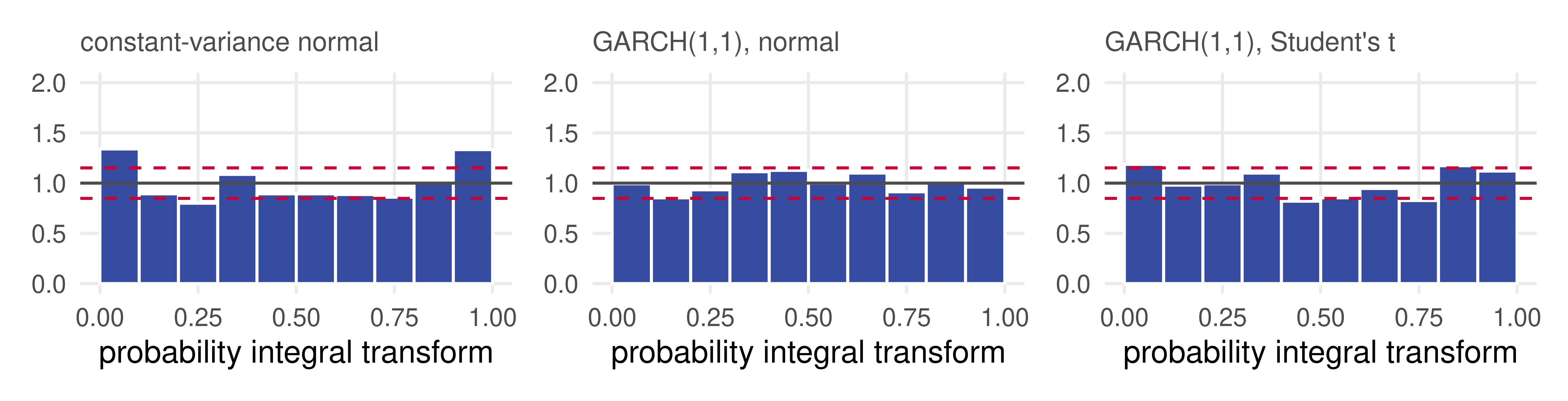
z <-list(constant =pnorm(yr, cm, cs), garch_normal =pnorm(yr, gn$Mu, gn$Sigma),garch_t =pdist("std", (yr - gt$Mu) / gt$Sigma, shape = gt$Shape))pit_plot(z$constant, sub ="constant-variance normal") |pit_plot(z$garch_normal, sub ="GARCH(1,1), normal") |pit_plot(z$garch_t, sub ="GARCH(1,1), Student's t")
Dashed lines: the band an iid uniform sample of this size respects bin by bin. Constant variance shows the butterfly, too many realizations in both tails: densities too thin-tailed. The GARCH densities are close to uniform; the t version leaves the outer deciles a little full.
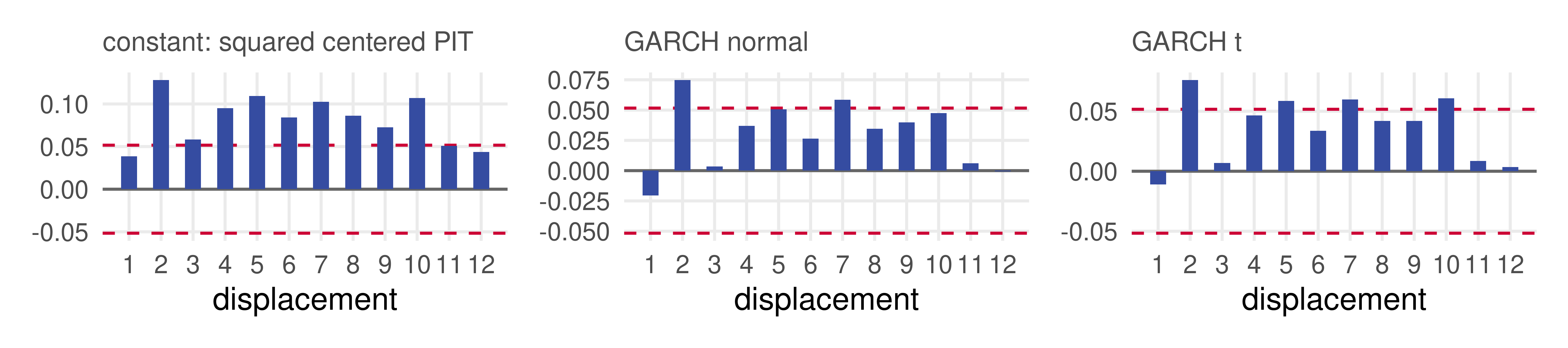
Under constant variance the squared PITs are strongly autocorrelated: neglected volatility dynamics show up as forecastable “errors”, as serial correlation does for point forecasts. GARCH halves the autocorrelations but does not remove them: refits only every 250 days leave some variance dynamics uncaptured.
Diebold runs the same sequence on S&P 500 returns; the PITs themselves also keep a small first-order autocorrelation.
What to take away
Unforecastability. Optimal errors cannot be forecast from what was known at the time: unbiased, one-step white noise, h-step at most MA(h-1), variances rising to the unconditional variance, orthogonal to the information set. Test with t statistics (HAC or MA(h-1) disturbances), correlograms, and the Mincer-Zarnowitz regression; a rejection is a recipe for a better forecast.
Accuracy is loss and horizon specific. MSE = variance + bias^2; RMSE and MAE keep units; compare with the mean and no-change benchmarks (predictive R^2, Theil’s U), and remember that the series itself bounds what any forecast can do.
Diebold-Mariano: a t test on the loss differential with robust standard errors. Quantitative beat judgmental at OverSea; the AR(2) beat the spread model and tied the professionals for GDP.
Intervals and densities: hit sequences should be iid Bernoulli (Christoffersen), PITs iid uniform. Constant-variance intervals fail both ways on daily returns; GARCH with t shocks passes.
R cheat sheet
library(fpp3); library(sandwich); library(lmtest)# ---- absolute standards -----------------------------------------------------------------arima(e, order =c(0, 0, h -1)) # mean of h-step errors with MA(h-1) disturbancescoeftest(lm(e ~1), vcov =NeweyWest(lm(e ~1), lag = h -1, prewhite =FALSE)) # HAC t test of zero meanhac_t(e, lag = h -1) # the same, one number (defined in these slides)correlogram(e, m =12); Box.test(e, 12, "Ljung-Box") # white noise / MA(h-1) checksmz_test(y, f, lag = h -1) # Mincer-Zarnowitz: y on f, Wald test of (0, 1)# ---- relative standards -----------------------------------------------------------------c(ME =mean(e), RMSE =sqrt(mean(e^2)), MAE =mean(abs(e))) # accuracy measures1-sum(e^2) /sum(e_mean^2); 1-sum(e^2) /sum(e_nochange^2) # predictive R2; Theil's Uhac_t(e1^2- e2^2, lag = h -1) # Diebold-Mariano statistic by regressionforecast::dm.test(e1, e2, h = h, power =2) # the packaged version; power = 1 for absolute lossaccuracy(fc, data) # fable: RMSE, MAE, MAPE, MASE for a fable of forecasts# ---- interval and density forecasts -----------------------------------------------------hit <-abs(y - f) <1.96* sigma; mean(hit); lr_uc(hit, 0.95); lr_ind(hit) # coverage and Christoffersen testsz <-pnorm(y, mu, sigma); pit_plot(z); acf_plot((z -mean(z))^2) # PITs, histogram, dependenceugarchroll(spec, r, n.ahead =1, forecast.length =1500, refit.every =250) # rolling GARCH density forecasts
References
Additional resources
Textbooks
Diebold, F.X. Forecasting in Economics, Business, Finance and Beyond, the chapters on evaluating point forecasts and on evaluating interval and density forecasts. The OverSea Shipping data come from the companion files of the book’s predecessor, Elements of Forecasting.
Hyndman, R.J. and Athanasopoulos, G. Forecasting: Principles and Practice (3rd ed.), the forecaster’s toolbox chapter, for accuracy measures (including MASE) and time series cross-validation in fable.
Original sources
Mincer, J. and Zarnowitz, V. (1969), “The Evaluation of Economic Forecasts,” in Economic Forecasts and Expectations, NBER. Theil, H. (1966), Applied Economic Forecasting, North-Holland.
Diebold, F.X. and Mariano, R.S. (1995), “Comparing Predictive Accuracy,” Journal of Business and Economic Statistics, 13, 253–263; Diebold, F.X. (2015), “Comparing Predictive Accuracy, Twenty Years Later,” JBES, 33, 1–9. West, K.D. (1996), Econometrica, 64, 1067–1084; Clark, T.E. and McCracken, M.W. (2001), Journal of Econometrics, 105, 85–110; Giacomini, R. and White, H. (2006), Econometrica, 74, 1545–1578.
Diebold, F.X. and Kilian, L. (2001), “Measuring Predictability: Theory and Macroeconomic Applications,” Journal of Applied Econometrics, 16, 657–669.
Christoffersen, P.F. (1998), “Evaluating Interval Forecasts,” International Economic Review, 39, 841–862. Diebold, F.X., Gunther, T.A. and Tay, A.S. (1998), “Evaluating Density Forecasts with Applications to Financial Risk Management,” International Economic Review, 39, 863–883.
Data: data/shipping_volume.csv (OverSea, 499 weeks); data/hw2_gdp_spread.csv (GDP growth and term spread, 1959Q1 to 2024Q2); data/spf_median_rgdp_growth.csv (Survey of Professional Forecasters, Federal Reserve Bank of Philadelphia); data/nyse_returns.csv.