Every model in this course has forecast a series from its own past: trend, seasonal, autoregression, GARCH. Yet economic variables move together. Housing completions follow housing starts, consumption follows income, inflation follows money growth, with leads and lags that are exactly what a forecaster wants to exploit.
Regression brings other variables in, but it labels one of them “dependent” and the rest “explanatory”, as if the explanatory ones were handed to us from outside. Usually they are not: we need to forecast them too, and the dependent variable may help forecast them in turn.
Sims (1980): all variables are endogenous; admit it from the outset, and model them as a system in which each variable depends on the lagged values of all. That system is a vector autoregression.
Today: what a VAR is, how to estimate and forecast it, how to read it (predictive causality, impulse responses, variance decompositions), and whether it beats univariate models on US housing data.
Diebold, Forecasting in Economics, Business, Finance and Beyond, the chapter on vector autoregressions; Stock and Watson (2001) for a reader’s guide to VARs. The housing data come from the book’s companion files.
From distributed lags to vector autoregressions
Distributed lag models
A regression usable one step ahead has a lagged regressor: y_t = \beta_0 + \delta\, x_{t-1} + \varepsilon_t. Generalize to several lags of x,
y depends on a distributed lag of past x’s; the \delta_i are the lag weights, their pattern the lag distribution.
With many lags, OLS spends many degrees of freedom. Polynomial distributed lags (Almon) restrict \delta_i = a + bi + ci^2: N_x weights from three parameters, smooth but ad hoc.
Rational distributed lags, the device of the ARMA lecture, are less arbitrary: y_t = \dfrac{A(L)}{B(L)}\, x_t + \varepsilon_t, that is B(L)\, y_t = A(L)\, x_t + B(L)\, \varepsilon_t. Multiplying out brings lags of y into the model along with lags of x.
One way or another, lags of the dependent variable belong in a multivariate forecasting model.
Do not forget the own dynamics
The regressors may not capture all the dynamics in y. Two ways to allow for the rest, as in the assembling lecture:
They are related. Take one lag of x and an AR(1) disturbance, \varepsilon_t = \phi\, \varepsilon_{t-1} + v_t, and multiply the regression through by (1 - \phi L):
A model with y_{t-1}, x_{t-1} and x_{t-2} on the right and white noise errors, subject to the restriction that the coefficient on x_{t-2} is minus the product of the other two. The lagged-dependent-variable model is the more general of the two.
Whether to include lagged y’s or ARMA disturbances is usually a minor issue. What matters is to allow for own-variable dynamics somehow. Lagged dependent variables absorb residual serial correlation and can dramatically improve forecasts.
Transfer function models, y_t = \frac{A(L)}{B(L)} x_t + \frac{C(L)}{D(L)} \varepsilon_t, nest both; Diebold leaves them as an exercise.
All variables are endogenous
The distributed lag model still treats x as given. But x has a future too, which we need for any horizon beyond one; and if x helps forecast y, why should y not help forecast x?
So write an equation for every variable, each with lags of every variable on the right. Nothing is exogenous; the right-hand side is the same in each equation; and because everything on the right is lagged, the system is a forecasting model from the start.
How is the economy affected by unexpected events and changes in economic policy? What effects do interest rate hikes and tax reductions have on the production of goods and services, unemployment, inflation and investment?
The Nobel committee’s summary of Christopher Sims’s contribution (2011 prize, shared with Thomas Sargent). His 1980 paper “Macroeconomics and Reality” proposed VARs as the alternative to large structural models whose exogeneity assumptions he called incredible.
The VAR: specification, estimation, lag selection
The VAR(p)
A univariate AR(p) regresses one variable on p of its own lags. An N-variable vector autoregression of order p has N equations, each regressing one variable on p lags of itself and of every other variable. The bivariate VAR(1):
Iterating, \mathbf{Y}_t = \sum_{j=0}^{\infty} \mathbf{F}^j\, \mathbf{U}_{t-j}, which converges when every eigenvalue of \mathbf{F} lies inside the unit circle: the multivariate version of the root condition for an AR(p). Then the VAR has the moving-average representation
the object behind forecast errors and impulse responses. vars::roots() reports the moduli of the eigenvalues.
With unit roots in the system the levels VAR is still usable for forecasting (Sims, Stock and Watson, 1990), but the asymptotics change; many practitioners difference first, or impose cointegration.
Estimation: equation by equation
A VAR looks hard to estimate: many equations, many regressors. It is the opposite. Every equation has the same regressors, so OLS equation by equation is fully efficient: no gain from accounting for the correlation across equations (seemingly unrelated regression would return the identical estimates).
N ordinary least squares regressions, one per variable. Simple and numerically stable, which is why VARs are so popular, and why multivariate ARMA models, whose estimation is unwieldy, are not.
The disturbance covariance matrix is estimated from the residuals: \hat\Sigma = \frac{1}{T} \sum_t \hat{\boldsymbol{\varepsilon}}_t \hat{\boldsymbol{\varepsilon}}_t'.
The usual t and F statistics apply in large samples, exactly as for an autoregression.
The cost is parameters. Each equation has Np + 1 coefficients, so the system has N(Np + 1): 18 for two variables and four lags, 150 for six variables and four lags. VARs with many variables are a case for the shrinkage principle (Bayesian VARs), a later topic.
If different equations had different regressors (some lags excluded), seemingly unrelated regression would be needed for efficiency.
Choosing the lag length
The information criteria of the univariate lectures generalize, with the log residual variance replaced by the log determinant of the residual covariance matrix:
Adding up the equation-by-equation criteria would be right only if the shocks were uncorrelated across equations, which they rarely are; \ln|\hat\Sigma| accounts for the correlation.
Choose p to minimize AIC or SIC, computed on the same sample for every p. SIC again prefers smaller models.
vars::VARselect() tabulates AIC, SIC (there called SC), Hannan-Quinn and the final prediction error.
Then check the residuals: a multivariate Ljung-Box (Portmanteau) test, and each equation’s residual correlogram, as always.
Forecasting with a VAR
Wold’s chain rule, vector version
Everything on the right-hand side is lagged, so the one-step forecast is immediate, and longer horizons follow by recursion, exactly as for an AR(p):
\mathbf{y}_{T+1,T} = \mathbf{c} + \Phi_1 \mathbf{y}_T + \cdots + \Phi_p \mathbf{y}_{T-p+1}, \qquad
\mathbf{y}_{T+h,T} = \mathbf{c} + \sum_{i=1}^{p} \Phi_i\, \mathbf{y}_{T+h-i,T}, \qquad \mathbf{y}_{s,T} = \mathbf{y}_s \text{ for } s \leq T .
The h-step error is a moving average of future shock vectors, with covariance matrix
whose diagonal gives each variable’s h-step forecast error variance, hence interval forecasts y_{j,T+h,T} \pm 1.96\, \sqrt{[\Sigma_h]_{jj}} and, under normality, a multivariate normal density forecast.
Operational forecasts replace \mathbf{c}, \Phi_i, \Sigma by estimates. Note what is not needed: any assumption about which shock is which. Forecasting uses the VAR as estimated; the identification questions of the impulse-response section do not arise.
The \Psi_i follow from the \Phi_i by the same recursion as the \psi weights of an AR(p), with matrices in place of scalars.
Predictive causality
Granger causality
A notion of causality tailored to forecasting, from Granger (1969) and Sims (1972), built on two principles: a cause occurs before its effect, and a cause contains information about the effect not available elsewhere, in particular not in the effect’s own past.
Definition.y_iGranger-causesy_j if lagged y_i helps predict y_j over and above the lagged values of y_j (and of the other variables in the system). In a VAR(p) this means that at least one of the p coefficients on lags of y_i in the y_j equation is nonzero.
Test.H_0: all p coefficients on lags of y_i in the y_j equation are zero; an ordinary F test (or Wald \chi^2) of p exclusion restrictions. Block versions test whether a set of variables helps predict another set.
Caveats. (1) This is predictive causality, a statement about forecasts, not about mechanisms: Christmas card sales Granger-cause Christmas. (2) In a bivariate VAR, one-step noncausality implies noncausality at every horizon; with three or more variables it does not, because y_i may cause y_k which causes y_j. (3) Tests can suggest restrictions worth imposing, which sometimes improves forecasts.
In the unrestricted VAR everything causes everything by construction; the test asks whether the data support the restriction that something does not.
Which came first?
Thurman and Fisher (1988) put the question to annual US data on chicken population and egg production, 1930 to 1983, with three lags:
data("ChickEgg", package ="lmtest")grangertest(chicken ~ egg, order =3, data = ChickEgg)$`Pr(>F)`[2] # do eggs help predict chickens?
## [1] 0.002966397
grangertest(egg ~ chicken, order =3, data = ChickEgg)$`Pr(>F)`[2] # do chickens help predict eggs?
## [1] 0.6237862
Lagged eggs help forecast chickens (p = 0.003); lagged chickens do not help forecast eggs (p = 0.62). Eggs Granger-cause chickens, not the reverse: the egg came first.
grangertest() runs the F test from two regressions, with and without the lags of the other variable. For a full system, vars::causality() does the same from a fitted VAR, as below.
Thurman, W.N. and Fisher, M.E. (1988), “Chickens, Eggs, and Causality, or Which Came First?”, American Journal of Agricultural Economics, 70, 237–238. A joke with a serious point: the test is about predictive content, nothing more.
Impulse responses and variance decompositions
Impulse responses: the univariate case
How does a unit shock affect a series, now and in the future? Read the answer off the moving-average representation. For the AR(1), y_t = \varepsilon_t + \phi \varepsilon_{t-1} + \phi^2 \varepsilon_{t-2} + \cdots, a unit shock to \varepsilon_t moves y by 1, \phi, \phi^2, \ldots: the impulse-response function.
the same process, now driven by a shock in standard deviation units. The response to a typical shock is \{\sigma, \phi\sigma, \phi^2\sigma, \ldots\}: b_0 = \sigma is the impact effect, b_1 the effect one period later, and so on. A one-standard-deviation shock is the natural experiment, because “one unit” of \varepsilon means nothing without knowing its scale.
Any multiple m gives an equivalent representation with b_i' = b_i m and \varepsilon_t' = \varepsilon_t / m; m = \sigma is the convenient choice.
Multivariate: the problem of correlated shocks
For the bivariate VAR(1), back substitution gives the moving-average form
The question is now “how does a shock to \varepsilon_i affect y_j, now and later, for every pair (i, j)?”
But the shocks are correlated: \sigma_{12} \neq 0. Moving \varepsilon_1 while holding \varepsilon_2 fixed is not an experiment the data ever perform; when \varepsilon_1 jumps, \varepsilon_2 typically jumps too. We first need shocks that are uncorrelated, then trace out their effects.
Decompose the second shock into the part explained by the first and an orthogonal remainder:
Substituting into the y_2 equation puts \frac{\sigma_{12}}{\sigma_1^2}\, y_{1,t} on its right-hand side: a contemporaneous effect of y_1 on y_2, with y_1 unaffected by y_2 within the period. That is a recursive (Cholesky) ordering, y_1 first.
Cholesky orthogonalization and ordering
In general, write \boldsymbol{\varepsilon}_t = P\, \mathbf{v}_t with \mathbf{v}_t \sim WN(\mathbf{0}, I) and P the lower-triangular Cholesky factor of \Sigma, PP' = \Sigma. Then
and the (j, i) element of \Psi_h P is the response of y_j, h periods later, to a one-standard-deviation shock v_i: the orthogonalized impulse-response function.
The shocks \mathbf{v}_t are uncorrelated and in standard deviation units: the univariate normalization carried over.
P is lower triangular, so the first variable responds on impact only to v_1, the second to v_1 and v_2, and so on. The ordering of the variables matters: it encodes who moves whom within the period. Order by economic reasoning, and check that the conclusions survive reversing it.
Point estimates of the responses replace parameters by estimates; confidence bands (by bootstrap) are routine in software but were long an open problem.
Hamilton (1994) gives the full treatment. Ordering and normalization affect only impulse-response analysis; forecasting needs the unorthogonalized model.
Variance decompositions
The same orthogonalized shocks answer a second question with an immediate forecasting meaning: what fraction of the h-step forecast error variance of y_j is due to shocks to y_i?
From \Sigma_h = \sum_{i=0}^{h-1} \Psi_i P P' \Psi_i', the h-step error variance of y_j is a sum of contributions, one per orthogonalized shock,
[\Sigma_h]_{jj} = \sum_{i=1}^{N} \underbrace{\sum_{s=0}^{h-1} \big([\Psi_s P]_{ji}\big)^2}_{\text{due to shock } i},
and the shares sum to one. Plotted against h for every (j, i) pair, this is the forecast error variance decomposition.
Impulse responses and variance decompositions present the same information in two ways, like correlograms and information criteria do for model selection. Impulse responses have become the more popular; the decomposition speaks the language of forecast error variance directly.
vars::fevd() computes it from a fitted VAR.
Application: housing starts and completions
The data
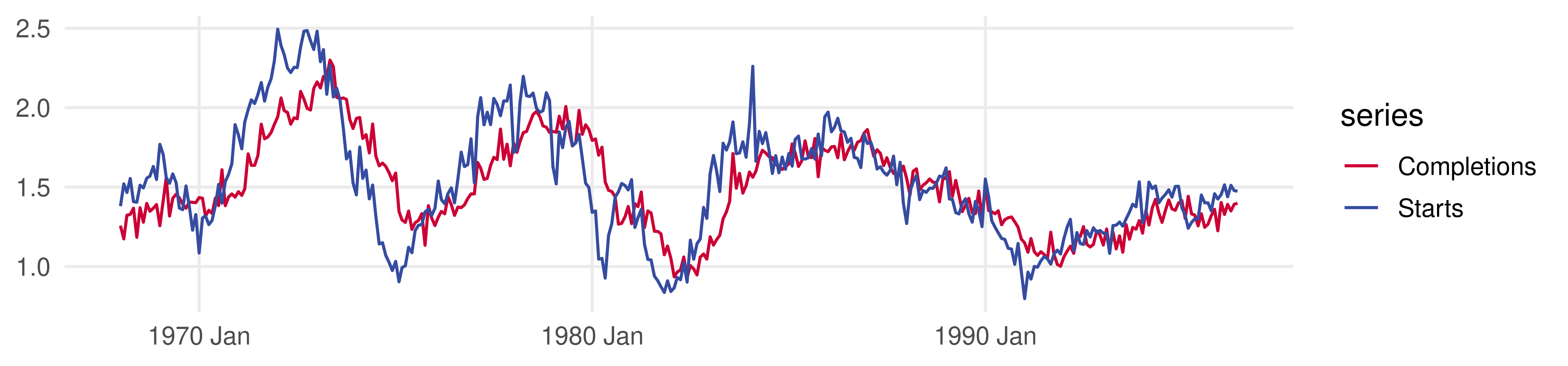
Monthly US housing starts and completions, seasonally adjusted, millions of units at annual rates, 1968M1 to 1996M6. Estimation on 1968M1 to 1991M12 (T = 288); 1992M1 to 1996M6 held out.
Both series are highly cyclical, and completions lag starts: it takes time to build a house.
Starts and completions, one at a time
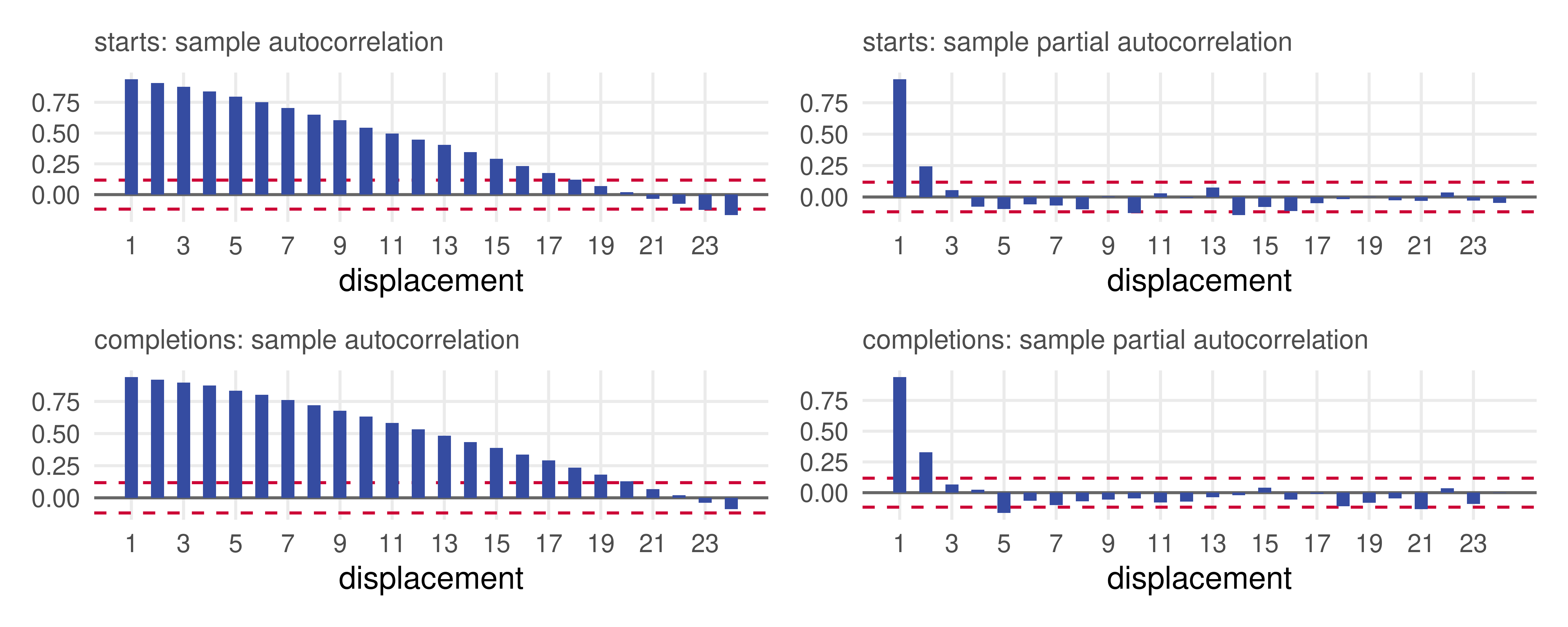
Each series alone looks like an AR(2): slowly decaying autocorrelations, partial autocorrelations that cut off after displacement 2, all highly significant.
The cross-correlation function
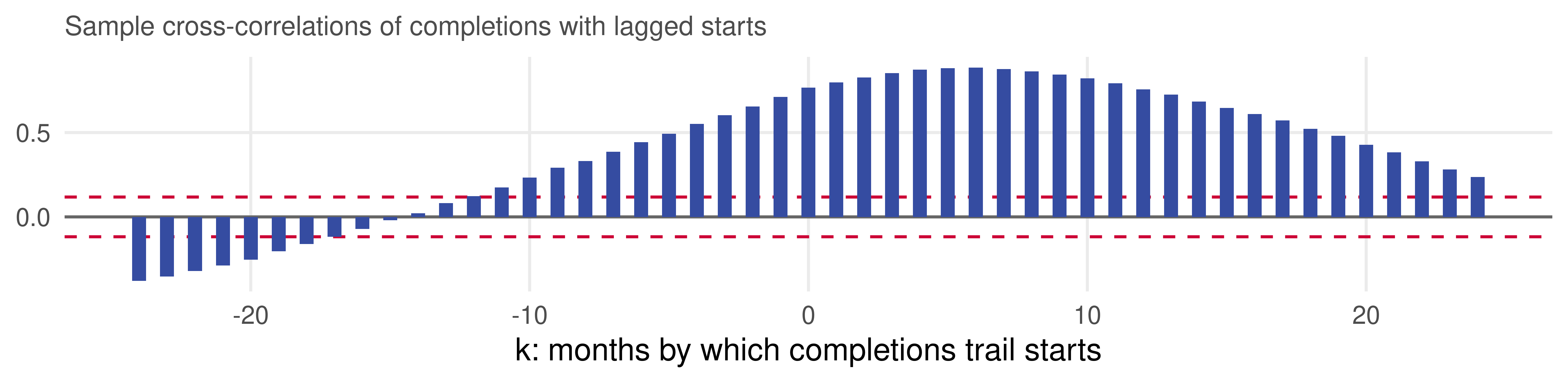
New in the multivariate setting: the correlation between one variable and lags of another, \rho_{yx}(\tau) = \operatorname{corr}(y_t, x_{t-\tau}), estimated the usual way and plotted against \tau with the same \pm 2/\sqrt{T} bands.
cc <-ccf(est$Completions, est$Starts, lag.max =24, plot =FALSE) # corr(completions_{t+k}, starts_t) at lag k
Starts and completions are highly correlated at every displacement. The contemporaneous correlation is 0.77; completions are most correlated with starts lagged about six months (0.89), the time it takes to build. The asymmetry is the first hint of causality running from starts to completions.
Lag selection and estimation
Y <- est |>as_tibble() |> dplyr::select(Starts, Completions) |>as.data.frame()VARselect(Y, lag.max =8, type ="const")$selection
## AIC(n)  HQ(n)  SC(n) FPE(n)
##      4      4      3      4
AIC and Hannan-Quinn pick four lags, SIC three. Following the book, we fit a VAR(4) by equation-by-equation OLS:
v4 <- vars::VAR(Y, p =4, type ="const") # fable also has a VAR(); vars:: picks the one meant hereround(coef(v4)$Completions, 3)
In the completions equation the first and fourth lags of starts are significant, and every own lag is. R^2 = 0.94, standard error 0.073, as in Diebold’s estimates.
round(cor(residuals(v4))[1, 2], 2) # correlation of the two equations' residuals
## [1] 0.18
Starts depend on their own past, with a long memory; no lag of completions has a significant effect on starts. Sensible: we expect starts to cause completions, not the reverse. The two equations’ shocks are only mildly correlated (0.18).
R^2 = 0.90, standard error 0.125, as in Diebold’s estimates.
Noncausality from starts to completions is rejected overwhelmingly (F = 26); from completions to starts only at the 6% level, weak evidence of feedback. The lagged starts in the completions equation are the information a univariate model throws away.
causality() also tests instantaneous causality, which concerns the residual correlation.
Impulse responses
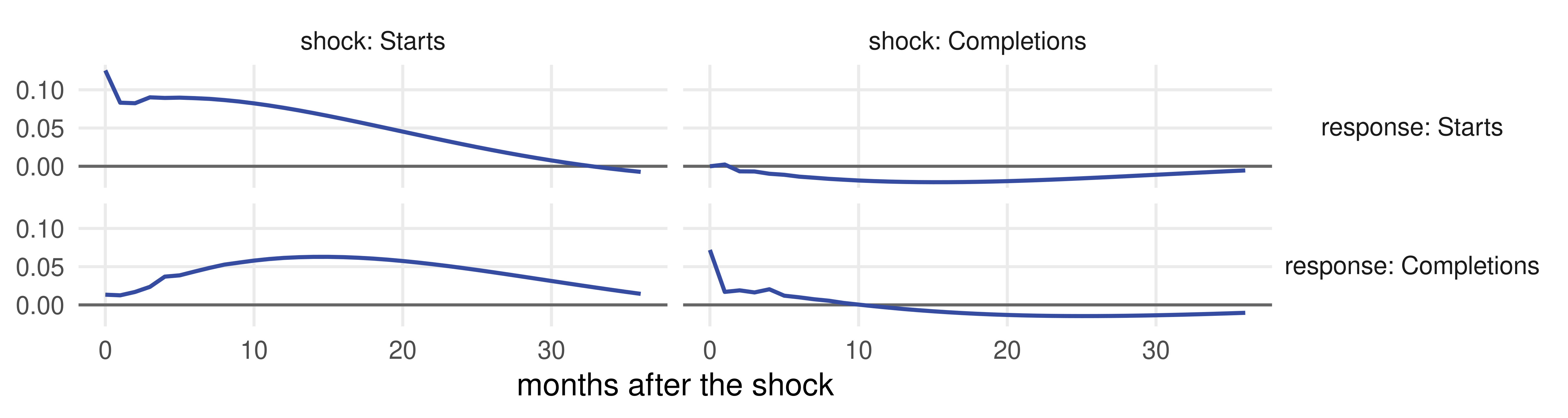
ir <-irf(v4, n.ahead =36, boot =FALSE) # orthogonalized (Cholesky) responses; Starts is ordered firstround(ir$irf$Starts[c(1, 16, 37), ], 3) # response to a one-sd starts shock at h = 0, 15, 36
Rows: responding variable; columns: shock. A starts shock moves completions more and more, peaking after fifteen months (time to build); a completions shock barely moves starts. Reversing the ordering changes nothing visible.
The forecast error variance of starts is essentially all due to its own shocks, at every horizon.
For completions, the share due to starts shocks is 3 percent one month ahead and rises to almost 90 percent at two years. Completions are, in the end, starts six to fifteen months earlier; in the short run they are their own past.
The remaining shares are due to completions shocks; each row’s shares sum to one.
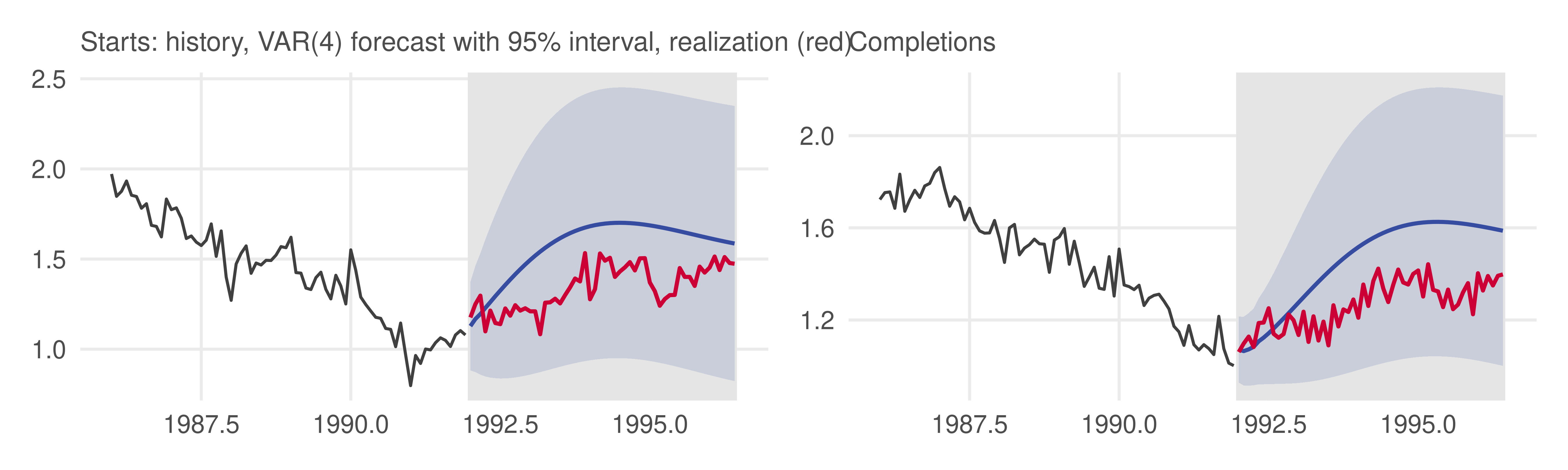
Starts had begun to recover before 1992 and the VAR projects the recovery to continue, faster than it did. Completions had not yet turned by 1991M12, yet the forecast calls the turning point correctly: the lagged starts already in the information set say so.
Does the VAR forecast better?
VAR(4) against two AR(4)s
The obvious competitor is a univariate AR(4) for each series, estimated on the same sample. Mean squared forecast errors over the 54 held-out months, by horizon:
ar4 <-lapply(c("Starts", "Completions"), function(v) as.numeric(predict(arima(est[[v]], order =c(4, 0, 0)), n.ahead =54)$pred))mse <-function(actual, fc, i) mean((actual[i] - fc[i])^2)blocks <-list(`h = 1 to 6`=1:6, `1 to 12`=1:12, `13 to 54`=13:54, `all 54`=1:54)round(rbind(`starts: VAR(4)`=sapply(blocks, mse, actual = hold$Starts, fc = pr$fcst$Starts[, "fcst"]),`starts: AR(4)`=sapply(blocks, mse, actual = hold$Starts, fc = ar4[[1]]),`completions: VAR(4)`=sapply(blocks, mse, actual = hold$Completions, fc = pr$fcst$Completions[, "fcst"]),`completions: AR(4)`=sapply(blocks, mse, actual = hold$Completions, fc = ar4[[2]])), 4)
##                     h = 1 to 6 1 to 12 13 to 54 all 54
## starts: VAR(4)          0.0101  0.0245   0.0770 0.0654
## starts: AR(4)           0.0089  0.0049   0.0073 0.0068
## completions: VAR(4)     0.0025  0.0032   0.0639 0.0504
## completions: AR(4)      0.0100  0.0122   0.0180 0.0167
Diebold poses exactly this comparison as an exercise. Univariate AR(4)s by exact maximum likelihood; the picture is the same with AIC-selected orders.
Reading the comparison
Completions, first year. The VAR’s error is a quarter of the AR’s. Lagged starts are informative about completions, as the causality test said, and the VAR used them to call the turning point that the univariate model missed.
Starts. No gain at any horizon, and a loss: completions do not cause starts, so the eight extra coefficients add only estimation noise.
Long horizons. The VAR loses on both series. Its forecasts revert quickly to the 1968 to 1991 mean of about 1.55 million starts; the 1990s recovery was slower and never got there. The parsimonious AR(4) reverts more slowly and happens to be closer.
Three lessons that recur throughout forecasting:
Cross-variable information helps where causality runs, and only there.
Richer models pay for their parameters in sampling error, visible at long horizons.
The univariate model is the benchmark every multivariate model must beat, and often does not.
Shrinking VAR coefficients toward a univariate random-walk or AR prior (the Minnesota prior of Litterman, 1986) is the standard answer to lesson 2, and keeps the VAR’s advantage where lesson 1 applies.
The same in fable
fable::VAR() fits the same OLS system from a formula, selects the order by information criterion if asked, and forecasts:
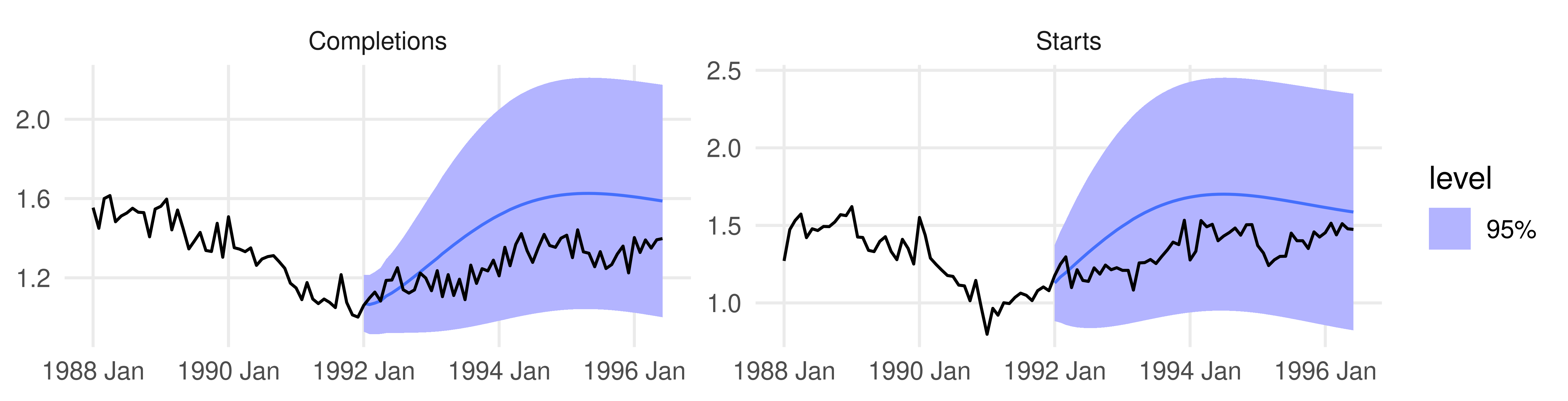
fv <- est |>model(VAR(vars(Starts, Completions) ~AR(4)))fv |>forecast(h =54) |>autoplot(hs |>filter(year(Month) >=1988), level =95) +labs(x =NULL, y =NULL)
AR(1:8) with ic = "bic" searches the order. tidy(fv) lists the coefficients, identical to vars::VAR()’s; the realizations in hs are drawn in black.
Beyond two variables: a macro VAR
Inflation, unemployment and the interest rate
Stock and Watson (2001) introduced VARs to a general audience with CPI inflation, the unemployment rate and the federal funds rate, quarterly, 1960 to 2000. Rebuilt from FRED-MD, averaging months by quarter:
##         cause
## equation  infl unemp  ffr
##    infl     NA     0 0.17
##    unemp 0.322    NA 0.05
##    ffr   0.000     0   NA
Inflation is predicted by past unemployment (the Phillips curve) but not by the interest rate.
Unemployment is predicted by the interest rate, marginally, and not by inflation.
The interest rate responds to both: the Fed moves rates when inflation and unemployment move. That is a Taylor rule read off the data.
Stock and Watson (2001) report the same pattern of p-values for 1960 to 2000. granger_matrix() is defined in the source of these slides; the information criteria prefer three lags here, and four changes nothing of substance.
Impulse responses to a monetary policy shock
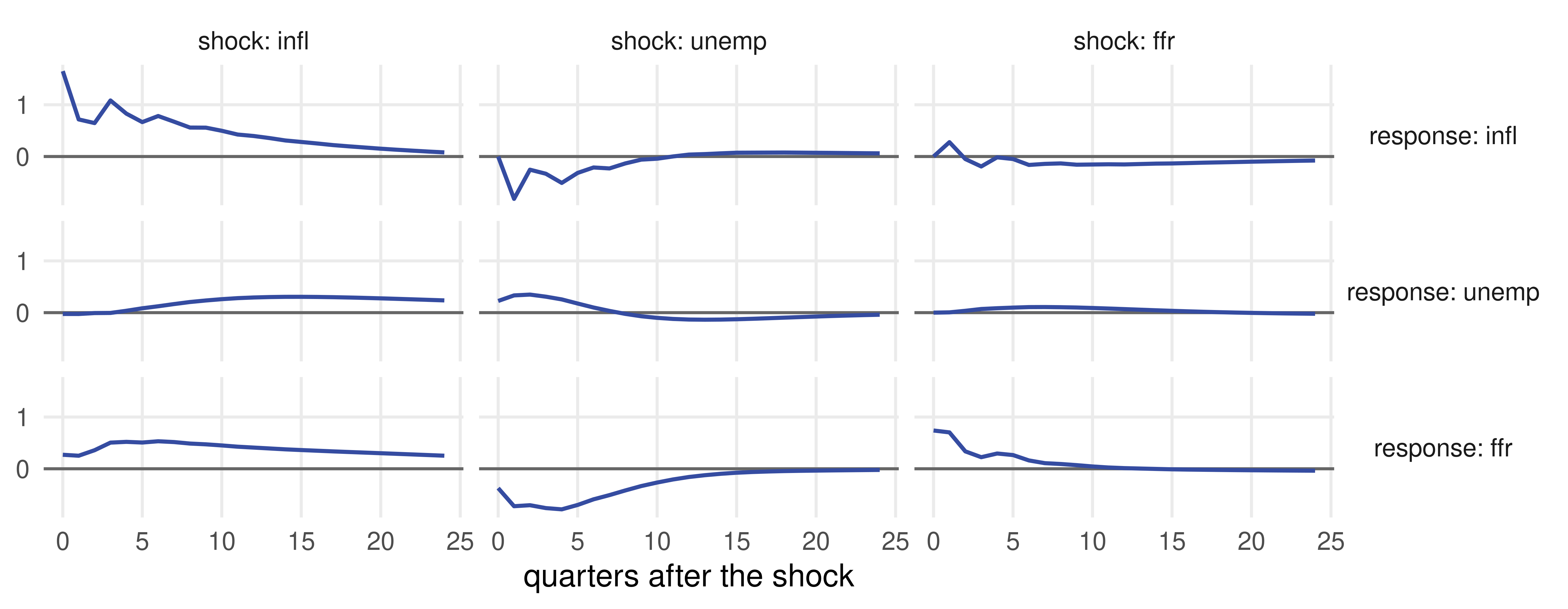
Ordering: inflation, unemployment, interest rate. The Fed is assumed to see current inflation and unemployment when it sets the rate, while the rate affects them only with a lag. Right column: an unexpected rate increase raises unemployment for about two years and lowers inflation after a year. Bottom row: the Fed cuts rates when unemployment rises and raises them when inflation rises.
What to take away
A VAR is N regressions with the same right-hand side: p lags of every variable. It captures cross-variable dynamics and correlated shocks that univariate models miss, is estimated by OLS equation by equation, and its order is chosen by multivariate AIC or SIC.
Forecasting is the chain rule with matrices; no identifying assumptions are needed.
Granger causality is predictive content: an F test of the lags of one variable in another’s equation. Eggs cause chickens; starts cause completions.
Impulse responses need orthogonal shocks, hence a Cholesky ordering that encodes who moves whom within the period; variance decompositions express the same information as shares of forecast error variance.
Housing. Starts lead completions by six to fifteen months. The VAR forecasts completions far better than a univariate model at short horizons and worse at long ones; for starts it never helps. Use cross-variable information where causality runs, and keep the univariate benchmark.
Macro. Three variables and four lags reproduce the Phillips curve, the Taylor rule and the lagged effect of monetary policy. The ordering is an assumption; the forecasts do not need it.
R cheat sheet
library(vars); library(lmtest); library(fpp3)# ---- specification and estimation --------------------------------------------------------ccf(y, x, lag.max =24, plot =FALSE) # cross-correlations corr(y_{t+k}, x_t)VARselect(Y, lag.max =8, type ="const")$selection # AIC, HQ, SC, FPE choices of pfit <- vars::VAR(Y, p =4, type ="const") # equation-by-equation OLS; Y a data frame of the seriescoef(fit)$Completions; summary(fit); roots(fit) # one equation's table; everything; companion rootsserial.test(fit, lags.pt =12, type ="PT.asymptotic") # multivariate Ljung-Box on the residuals# ---- reading the system -----------------------------------------------------------------causality(fit, cause ="Starts")$Granger # F test: do lags of Starts matter in the other equations?grangertest(y ~ x, order =3, data = d) # the bivariate version from two regressions (lmtest)irf(fit, n.ahead =36, boot =FALSE) # orthogonalized impulse responses, variables in column orderfevd(fit, n.ahead =36) # forecast error variance decompositions# ---- forecasting ------------------------------------------------------------------------predict(fit, n.ahead =54)$fcst$Starts # point forecasts and 95% bounds, by the chain ruletsb |>model(VAR(vars(y1, y2) ~AR(4))) |>forecast(h =54) # fable; AR(1:8) with ic = "bic" to select p
References
Additional resources
Textbooks
Diebold, F.X. Forecasting in Economics, Business, Finance and Beyond, the chapter on vector autoregressions. The housing application and its data come from the book’s companion files.
Hamilton, J.D. (1994), Time Series Analysis, and Lütkepohl, H. (2005), New Introduction to Multiple Time Series Analysis, Springer, for the full theory. Kilian, L. and Lütkepohl, H. (2017), Structural Vector Autoregressive Analysis, Cambridge, for identification.
Stock, J.H. and Watson, M.W. (2001), “Vector Autoregressions,” Journal of Economic Perspectives, 15, 101–115. Litterman, R.B. (1986), Journal of Business and Economic Statistics, 4, 25–38, on Bayesian VARs.
Sims, C.A., Stock, J.H. and Watson, M.W. (1990), Econometrica, 58, 113–144, on VARs with unit roots. Thurman, W.N. and Fisher, M.E. (1988), American Journal of Agricultural Economics, 70, 237–238.
Software: Pfaff, B. (2008), “VAR, SVAR and SVEC Models: Implementation within R Package vars,” Journal of Statistical Software, 27(4).
Data: data/housing_starts_completions.csv, US housing starts and completions, monthly 1968M1 to 1996M6, from the companion files; lmtest::ChickEgg; data/2024-07-fredmd.csv (CPIAUCSL, UNRATE, FEDFUNDS) for the macro VAR.