In the trend and seasonality lecture a trend was a deterministic function of time: a line, a parabola, an exponential. Extrapolating it was trivial, and the forecast error variance never grew with the horizon.
In the lecture on assembling the components, the liquor sales forecasts missed because the trend bent. The model that fitted 26 years of data had no way to know that the next two would be different.
For many economic series a different description fits better: the trend itself is random, a cumulation of shocks that never die out. Such a series has a unit root, or a stochastic trend, and it changes everything about forecasting it.
Today: random walks, integrated series, what they do to forecasts and to regressions, and how to test for a unit root.
Diebold’s Elements of Forecasting (the chapter on unit roots and stochastic trends); Hamilton (1994); Hyndman and Athanasopoulos, FPP3 (the ARIMA chapter). The yen/dollar data come from the Elements companion files.
Random walks
The random walk
Set \phi = 1 in the AR(1), y_t = \phi\, y_{t-1} + \varepsilon_t with \varepsilon_t \sim \text{iid}(0, \sigma^2):
y_t = y_{t-1} + \varepsilon_t .
Tomorrow’s value is today’s plus an unpredictable step. The root of 1 - L is L = 1, on the unit circle: hence “unit root”. The stationarity condition fails, just barely.
set.seed(1); n <-200; e <-matrix(rnorm(n *4), n) # four shock sequencesrw <-apply(e, 2, cumsum) # four random walksar <-apply(e, 2, function(v) stats::filter(v, 0.95, "recursive")) # four AR(1) paths, same shocks
Same shocks, left and right. The stationary paths keep returning to zero; the random walks wander off and stay away.
Properties
With y_0 = 0, back substitution gives y_t = \varepsilon_1 + \varepsilon_2 + \cdots + \varepsilon_t: today’s level is the sum of every shock that ever hit. Shocks are permanent.
The variance grows without bound and the autocovariances depend on t, not just on \tau: not covariance stationary, so none of the stationary theory applies. The usual laws of large numbers and central limit theorems are gone as well.
For large t the correlation between y_t and y_{t-\tau} is close to one at every moderate \tau. The sample autocorrelation function of a random walk starts near 1 and decays linearly and slowly: the signature we met in the ACF of log GDP.
Economics: if asset prices followed random walks, no information in past prices would help forecast future prices. That is the efficient markets hypothesis of Samuelson (1965) and Fama (1970).
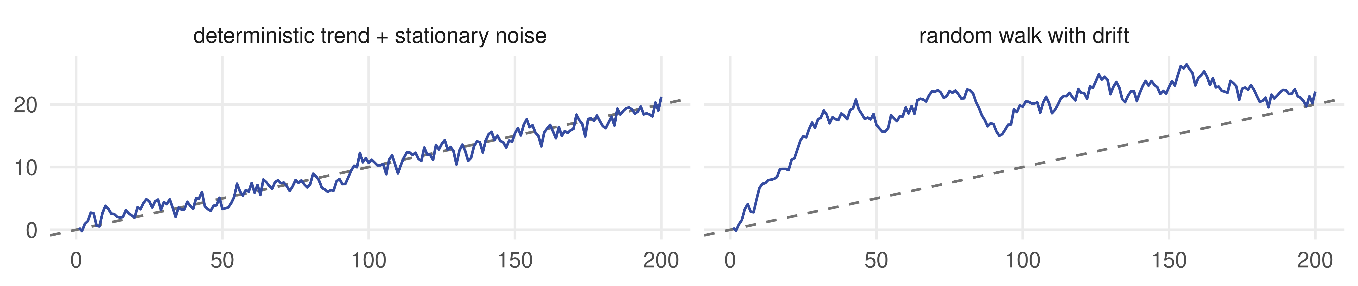
The series trends upward at rate \mu on average, but the stochastic trend makes it wander ever farther from the line \mu t. Forecasts: y_{T+h,T} = y_T + \mu h, a straight line from the last observation, with \sigma_h^2 = h\sigma^2 as before.
Same drift \mu = 0.1, same shocks, dashed line \mu t in both panels. Both series “trend”, for entirely different reasons.
Trend stationary or difference stationary?
Two models of a trending series, and two cures:
Trend stationary
Difference stationary
Model
y_t = \beta_0 + \beta_1 t + u_t, u_t stationary
\Delta y_t = \mu + u_t, u_t stationary
The trend is
a fixed line; deviations are temporary
a random walk; deviations are permanent
To make stationary
regress on time, keep the residual (detrend)
take first differences (difference)
Long-horizon forecast
returns to the line \beta_0 + \beta_1 (T+h)
a line from y_T with slope \mu
Interval width as h \to \infty
converges to \pm 1.96\, \sigma_u
grows like \sqrt{h} without bound
The trend and seasonality lecture assumed the left column. If the truth is the right column, detrending leaves a random walk in the residual, and the forecast reverts to a line the series has no reason to return to, with intervals that are far too narrow. Both mistakes compound at long horizons, which is exactly where trend forecasts are used.
Integrated series and ARIMA models
Orders of integration
A stationary series (loosely, one whose dependence dies out) is integrated of order zero, I(0).
A series whose first difference \Delta y_t = y_t - y_{t-1} is I(0) is integrated of order one, I(1). The random walk, with or without drift, is the leading case: \Delta y_t = \mu + \varepsilon_t.
I(d): the d-th difference \Delta^d y_t is stationary. In economics and finance d is 0, 1 or occasionally 2 (price levels when inflation itself has a unit root).
Where the unit root sits: the autoregressive polynomial factors as \Phi(L) = (1 - L)\, \Phi^*(L) with the remaining roots of \Phi^*(L) outside the unit circle. Then
\Phi^*(L)\, (1 - L)^d\, y_t = c + \Theta(L)\, \varepsilon_t
is an ARIMA(p, d, q): an ARMA(p, q) for the d-th difference. The I stands for integrated, because y_t is obtained by summing (integrating) the stationary series d times.
\Phi(1) = 0 is the algebraic statement of a unit root: 1 - \phi_1 - \cdots - \phi_p = 0, the boundary of the quick stationarity check of the cycles lecture.
Simulating and fitting an ARIMA
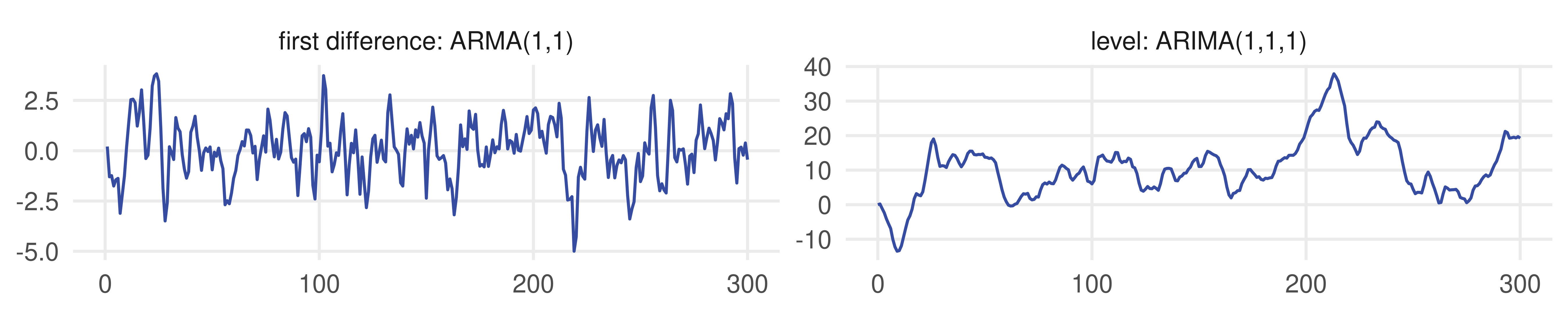
set.seed(5); z <-arima.sim(n =300, list(order =c(1, 1, 1), ar =0.5, ma =0.4)) # 301 values, z_0 = 0d <-rbind(data.frame(t =0:300, series ="level: ARIMA(1,1,1)", y =as.numeric(z)),data.frame(t =1:300, series ="first difference: ARMA(1,1)", y =as.numeric(diff(z))))ggplot(d, aes(t, y)) +geom_line(colour = smu_blue) +facet_wrap(~ series, scales ="free_y") +labs(x =NULL, y =NULL)
coef(arima(z, order =c(1, 1, 1))) # d = 1: the ARMA is fit to the differences
##       ar1       ma1
## 0.5017037 0.4137805
In fable, ARIMA(y ~ pdq(1, 1, 1)); ARIMA(y) alone chooses d by a unit root test and p, q by AICc.
Forecasting an ARIMA(p,1,q)
Forecast the stationary differences with the ARMA chain rule, then add them up:
The forecasts of \Delta y converge to the drift \mu, so the level forecast settles on a straight line with slope \mu starting from where the data left off, after a transition shaped by the ARMA dynamics.
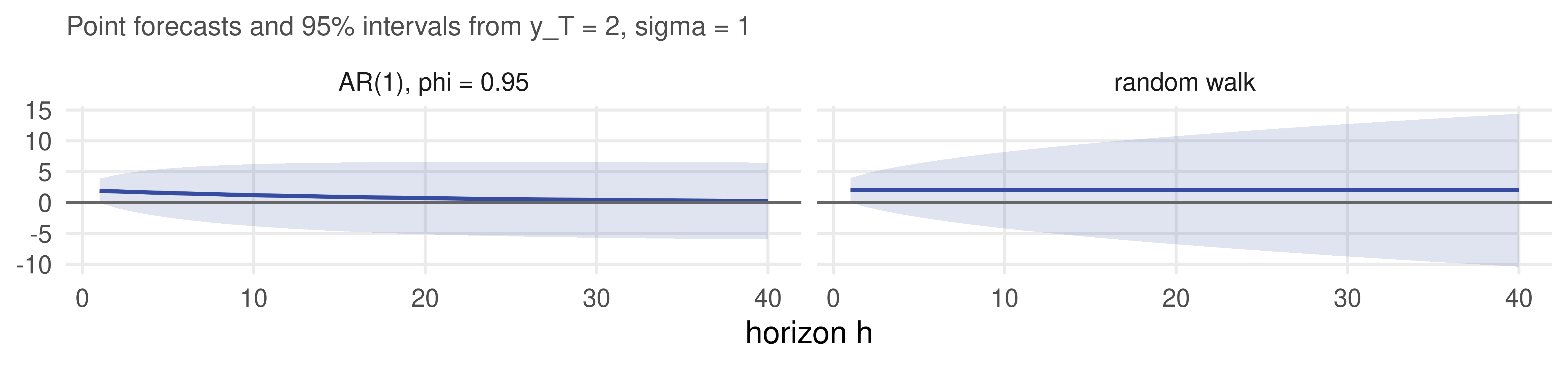
The forecast errors cumulate: \sigma_h^2 = \sigma^2 \sum_{i=0}^{h-1} \psi_i^2 with \psi_i now the moving-average weights of the level, which do not die out (\psi_i \to \Theta(1)/\Phi^*(1)). The variance grows roughly linearly in h forever.
Nothing about the forecasting procedure is new. The chain rule, the moving-average weights and the interval formula are those of the cycles lectures, applied to \Delta y and summed. What is new is the behavior of the result: no mean reversion, no bounded uncertainty.
With d = 2, the forecasts of \Delta y follow a line and the level forecast a parabola; this is one reason to be suspicious of d = 2.
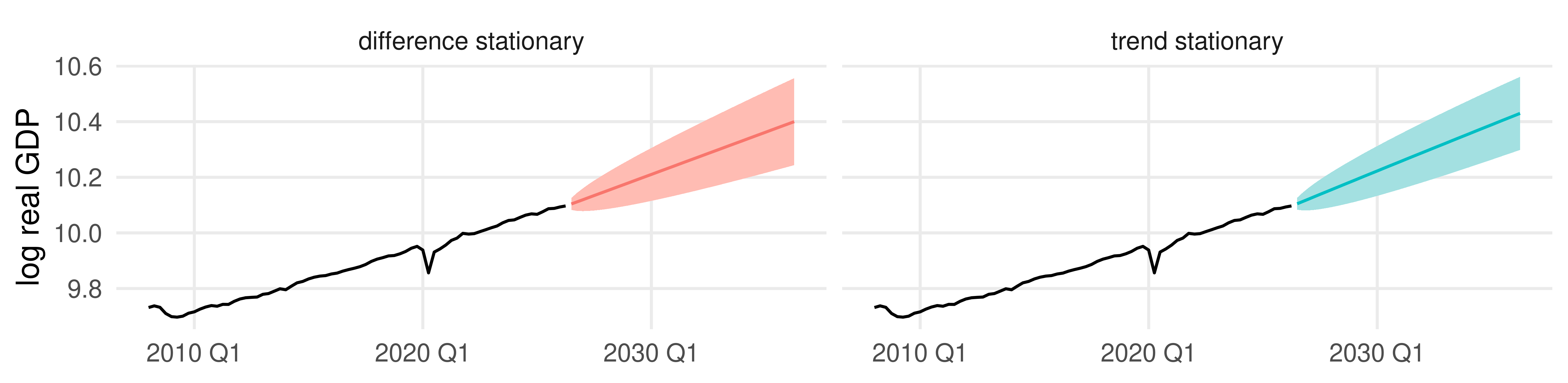
Quarterly, 1947Q1 to 2026Q2. Left: ARIMA(1,1,0) with drift. Right: AR(2) around a linear trend. The point forecasts are close over ten years, but one band keeps widening and the other stops. Which is honest? That is the testing question.
Why it matters: forecasts and regressions
Which model for the yen?
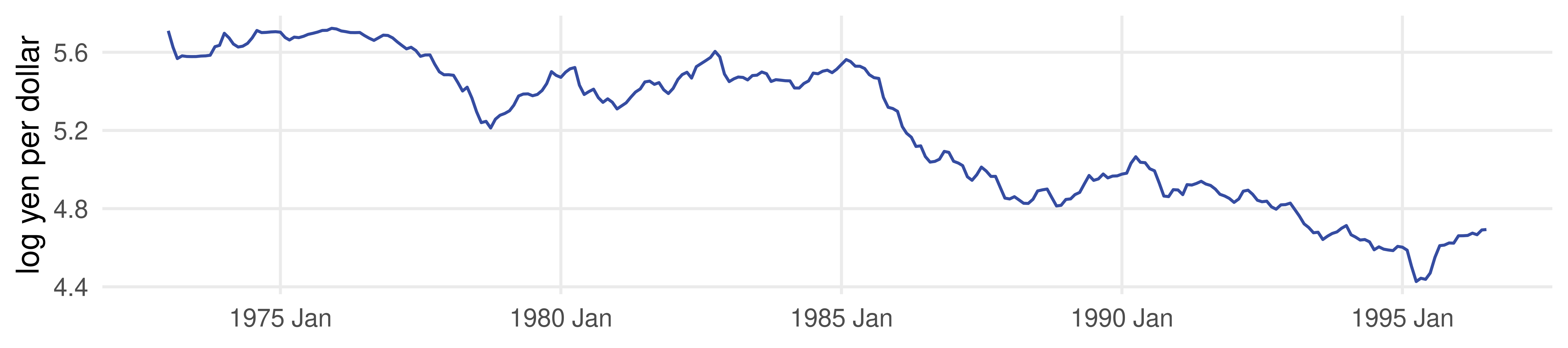
Monthly yen/dollar rate, 1973M1 to 1996M7, in logs. Estimate on 1973 to 1994, hold out 1995M1 to 1996M7.
ex <-read.csv("data/exchange_rates.csv") |>mutate(Month =yearmonth(Month), lyen =log(Yen)) |>as_tsibble(index = Month)est <- ex |>filter(year(Month) <=1994); hold <- ex |>filter(year(Month) >=1995)autoplot(ex, lyen, colour = smu_blue) +labs(x =NULL, y ="log yen per dollar")
A steady appreciation of the yen over two decades, from 300 to about 100 yen per dollar. A linear trend with a stationary cycle around it? Or a random walk with drift? Both describe the picture.
Diebold’s Elements of Forecasting, yen/dollar application; data/exchange_rates.csv.
In levels, AIC and SIC among ARMA(p,q)-plus-trend models pick an AR(2) (or an ARMA(1,1), a hair apart). Its AR coefficients sum to 0.97: inverse roots 0.95 and 0.36. The trend slope is -0.4 percent a month. A model that is almost, but not quite, a random walk with drift.
0 + removes the constant; with pdq(0, 1, 0) a constant is a drift. The first autocorrelation of \Delta \ln(\text{yen}) is 0.32, hence the ARIMA(0,1,1) candidate.
Forecasts and realization
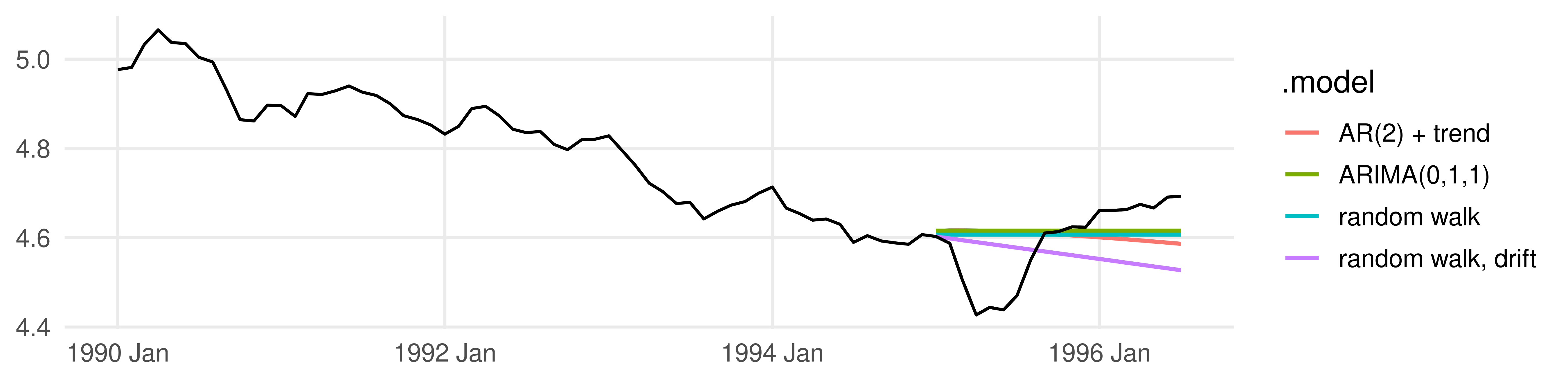
fc <- fits |>forecast(h =19)fc |>autoplot(ex |>filter(year(Month) >=1990), level =NULL, linewidth =0.8) +geom_line(data = hold, aes(Month, lyen), colour ="black", linetype ="longdash") +# the realizationlabs(x =NULL, y =NULL)
The AR(2) with trend continues the appreciation and then bends back toward its trend line; by five years out it would forecast 4.44, far below anything in the sample’s last decade.
The random walk says “stay where you are”: 4.61 at every horizon.
The realization (dashed) went the other way: the yen depreciated through 1995 and 1996.
## # A tibble: 4 × 3
##   .model               RMSE    MAE
##   <chr>               <dbl>  <dbl>
## 1 random walk        0.0895 0.0703
## 2 ARIMA(0,1,1)       0.0916 0.0697
## 3 AR(2) + trend      0.0971 0.0784
## 4 random walk, drift 0.109  0.0963
Every model was wrong, but the one that admitted it knew nothing about the direction was least wrong, and the one that extrapolated two decades of appreciation was worst. Diebold’s Elements reaches the same verdict: for the yen, difference, do not detrend.
The intervals tell the same story. The random walk’s 95% band at h = 19 is \pm 0.24 in logs, about \pm 27 percent, and the realization sits inside it. The trend-stationary band is about as wide at this horizon, because its dominant root is 0.95; further out it stops growing, and would eventually exclude where the yen actually went.
accuracy() compares the forecasts with the realizations held in ex. Exercise: redo this with the DM/dollar rate in the same file.
Spurious regression
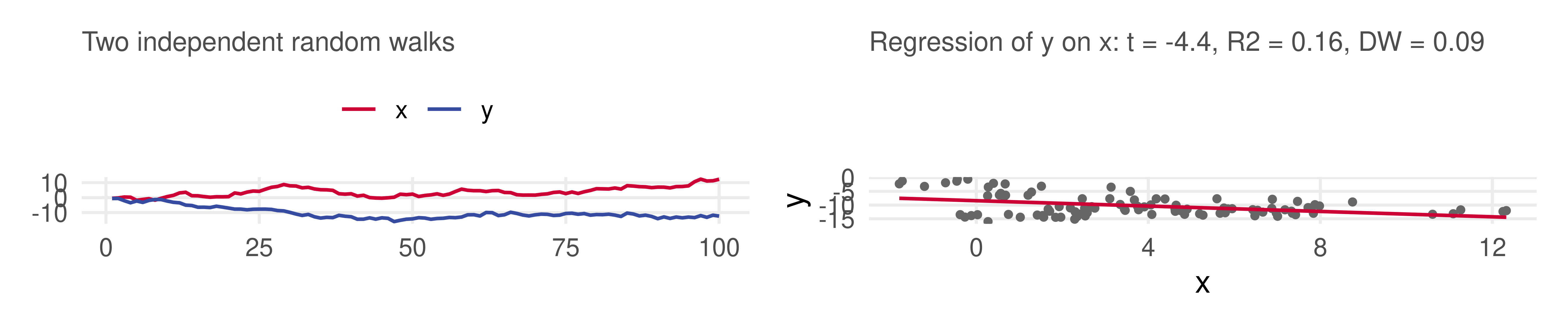
Two series that are completely unrelated, both random walks. Regress one on the other:
set.seed(2); R <-2000; n <-100one <-function(y, x) { f <-lm(y ~ x); e <-residuals(f)c(t =coef(summary(f))["x", "t value"], R2 =summary(f)$r.squared, DW =sum(diff(e)^2) /sum(e^2)) }spur <-replicate(R, one(cumsum(rnorm(n)), cumsum(rnorm(n)))) # independent random walksiid <-replicate(R, one(rnorm(n), rnorm(n))) # independent white noisesumm <-function(m) c(`P(|t| > 1.96)`=mean(abs(m["t", ]) >1.96), `median R2`=median(m["R2", ]),`median DW`=median(m["DW", ]))rbind(`random walks`=summ(spur), `white noise`=summ(iid))
##              P(|t| > 1.96)   median R2 median DW
## random walks        0.7585 0.168947027 0.1534009
## white noise         0.0545 0.004287033 1.9868108
With white noise the t test rejects 5% of the time, as it should. With random walks it rejects three times out of four, the R^2 is often substantial, and the Durbin-Watson statistic is near zero. Granger and Newbold (1974) called this spurious regression: two trending series look related because each wanders, and standard inference is simply invalid.
The t statistic does not converge at all; it diverges like \sqrt{T} (Phillips, 1986). More data make the problem worse.
Spurious regression, seen, and cured
Two remedies, both of which we have been preaching all along:
Allow for dynamics. Add y_{t-1} to the regression: the rejection rate falls to about 17%, still too high but no longer absurd. The low Durbin-Watson was the warning sign.
Difference. Regress \Delta y_t on \Delta x_t: both are white noise, and the rejection rate is 6%. Differencing is the standard cure, at the cost of throwing away the levels relationship.
When two I(1) series do share a stochastic trend, a regression in levels is meaningful (cointegration, Engle and Granger, 1987). That is a topic for a later course.
Stationarization in practice
Applied macroeconomists transform each series to stationarity before modeling. FRED-MD, the monthly database used earlier in the course, publishes a transformation code for every series:
tcode
1
2
3
4
5
6
7
transform
x_t
\Delta x_t
\Delta^2 x_t
\ln x_t
\Delta \ln x_t
\Delta^2 \ln x_t
\Delta (x_t / x_{t-1} - 1)
fm <-read.csv("data/2024-07-fredmd.csv", check.names =FALSE); tcode <-unlist(fm[1, -1]); fm <- fm[-1, ]tcode[c("INDPRO", "PAYEMS", "S&P 500", "CPIAUCSL", "FEDFUNDS", "GS10", "UNRATE", "HOUST")]
Output, employment and stock prices: growth rates (5). Interest rates and unemployment: changes (2). Prices (and money): changes in inflation (6), second differences of logs. Housing starts: logs only (4). The codes are the maintainers’ judgment about how many unit roots each series has.
McCracken and Ng (2016). Differencing changes the question as well as the statistics: a regression of \Delta y on \Delta x estimates a short-run relationship, not the one between the levels.
In a stationary autoregression t_\rho is approximately N(0,1) in large samples, and we would reject when t_\rho < -1.645. Under H_0 the regressor y_{t-1} is a random walk, its sum of squares grows like T^2 rather than T, and the normal approximation fails. Dickey and Fuller (1979) worked out what replaces it.
One-sided: explosive alternatives \rho > 1 are taken up at the end. s^2 is the usual residual variance.
The OLS estimate of \tau is \hat\rho - 1 and its t ratio is exactlyt_\rho: the same test, written as a regression of the change on the lagged level. Under H_0 the left-hand side is stationary and the right-hand side is not, which is what gives the statistic its odd distribution.
Every software package, urca included, reports the \tau form: the coefficient on z.lag.1 and its t value. Remember three things when reading the output:
the test is one-sided, and the statistic is usually negative;
compare it with the Dickey-Fuller critical values printed with it, not with -1.645;
more negative means more evidence against the unit root.
The Dickey-Fuller distribution, by simulation
The limiting distribution has no closed-form density, but it is trivial to approximate: generate random walks, run the regression, keep the t statistic, repeat.
set.seed(10); R <-10000t_null <-df_t(n =250, R = R) # df_t() is defined in the source of these slidesround(quantile(t_null, c(0.01, 0.05, 0.10, 0.50, 0.90)), 2)
The 5% critical value is about -1.95, not -1.645. Using the normal value, a test meant to have size 5% rejects a true unit root 10% of the time.
The distribution is shifted left: \hat\rho < 1 in about 69% of samples. OLS is biased toward stationarity under the null, the small-sample bias of the cycles lecture taken to its extreme.
Fuller’s (1976) tabulated values for this case: -2.58, -1.95 and -1.62 at 1%, 5% and 10%. The simulation takes under a second.
Null and alternative, side by side
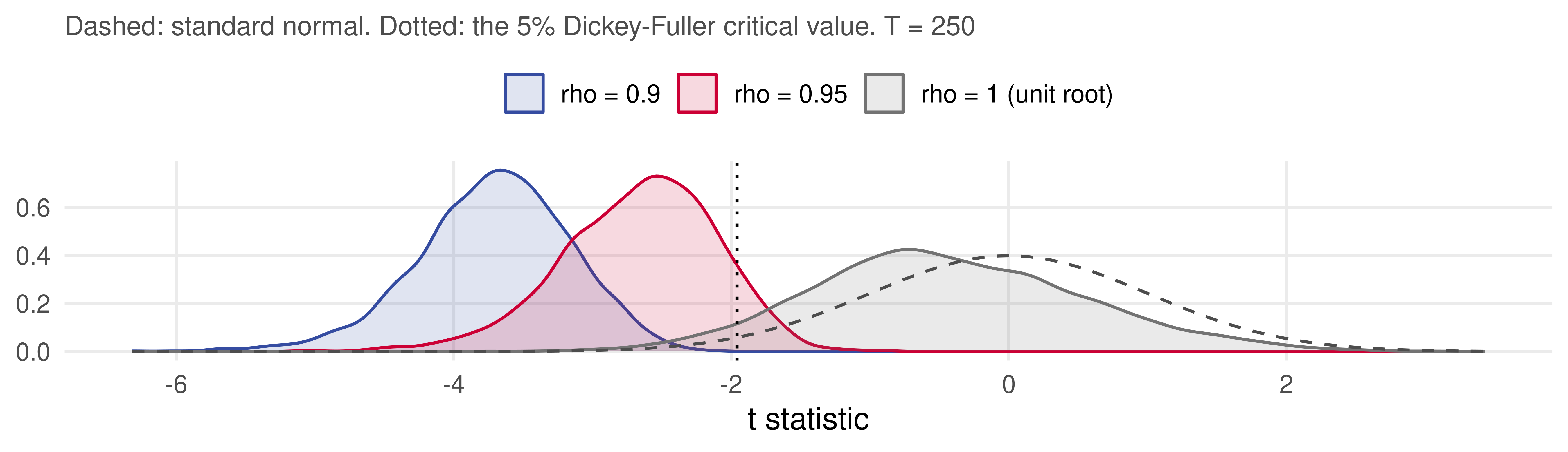
t_095 <-df_t(n =250, R =2000, rho =0.95); t_090 <-df_t(n =250, R =2000, rho =0.90)dd <-rbind(data.frame(case ="rho = 1 (unit root)", t = t_null), data.frame(case ="rho = 0.95", t = t_095),data.frame(case ="rho = 0.9", t = t_090))dens_plot(dd, cv =quantile(t_null, 0.05), # dens_plot() is in the sourcesub ="Dashed: standard normal. Dotted: the 5% Dickey-Fuller critical value. T = 250")
Under the null the density sits to the left of the normal. Under the alternatives it moves further left: at T = 250 the test rejects \rho = 0.95 in 92% of samples and \rho = 0.9 always.
Where the distribution comes from
For the curious. Under H_0, with W(r) a standard Brownian motion on [0, 1],
The partial sums T^{-1/2} \sum_{t \leq rT} \varepsilon_t behave like a Brownian motion, so sums of y_{t-1}^2 and of y_{t-1}\varepsilon_t converge to integrals of it (a functional central limit theorem).
\hat\rho converges at rate T, not \sqrt{T}: superconsistency. The regressor is so variable that the coefficient is pinned down very precisely, yet the t ratio is not normal.
The numerator equals \tfrac{1}{2}\big(W(1)^2 - 1\big), half a \chi^2_1 minus its mean. A \chi^2_1 is below its mean with probability 0.68: that is the leftward skew seen in the simulation.
Phillips (1987); Hamilton (1994). Nothing below depends on this slide, but it explains why every unit root test comes with its own table.
Power against roots near one
The same simulation at T = 100, with the alternative moved closer to the null:
Against \rho = 0.95 with 100 observations the test rejects about a third of the time; against \rho = 0.99 it almost never does. Unit root tests have low power against the alternatives that matter most in economics, where roots of 0.95 are common.
Power comes from the span of the data, not the number of observations: 100 years of annual data beat 25 years of monthly data for distinguishing \rho = 0.97 from 1.
So “cannot reject a unit root” is a weak statement. It is good practice to also run a test whose null is stationarity, which we do below.
In R: urca::ur.df
set.seed(3); rw <-cumsum(rnorm(200)); st <-as.numeric(arima.sim(list(ar =0.7), n =200))test_rw <-ur.df(rw, type ="none", lags =0); test_st <-ur.df(st, type ="none", lags =0)rbind(`random walk`= test_rw@teststat, `AR(1), phi = 0.7`= test_st@teststat); test_rw@cval
type = "none" is the regression of the last slides, no constant, no trend; lags = 0 adds no lagged differences (next section). @teststat is t_\tau and @cval the critical values to compare it with. summary() prints the whole regression.
The random walk gives -1.8, inside the acceptance region (the 5% critical value is -1.95); the stationary AR(1) gives -5.8 and is rejected at any level.
The critical values in urca come from Fuller’s tables and depend only on T and type, not on the data.
Drift and trend: which regression?
Three regressions
The regression of \Delta y_t on y_{t-1} can include deterministic terms, and the distribution of t_\tau changes with them:
A constant and a trend push the distribution further left: a given t_\tau is weaker evidence. Fuller’s tables give -2.86 and -3.41 at 5%.
urca labels the statistics tau1, tau2, tau3, and adds F tests of the joint hypotheses (phi1, phi2, phi3), each with its own table.
Choosing the specification
The deterministic terms are nuisance parameters, but the choice matters: too few and the test is badly sized when the data trend; too many and power is lost.
If the series shows no trend and a nonzero mean (an interest rate, an unemployment rate, a ratio): type = "drift".
If the series trends (log GDP, log prices, log stock indices): type = "trend". Under H_0 it is a random walk with drift; under H_1 it is trend stationary. Both describe trending data, so the test asks the right question.
type = "none" only when the mean is known to be zero, which is rare outside returns and residuals.
Rule of thumb: fit the specification that is a plausible description of the data under both hypotheses. With the "trend" type, a random walk without drift is still allowed under H_0; the reverse is not true. Sequential procedures that test the deterministic terms as well exist (Elder and Kennedy, 2001), but graphing the series usually settles it.
Example: the yen
yen_df <-ur.df(est$lyen, type ="trend", lags =3)rbind(statistic = yen_df@teststat); yen_df@cval
t_\tau = -2.50 against a 5% critical value of -3.42 (10%: -3.13): we cannot reject a unit root in the log yen/dollar rate. The joint test phi3 of a unit root and no trend (\delta = \tau = 0) is 3.5, below its 5% value of 6.3: not rejected either. The data are consistent with a random walk without drift, which is the model that forecast best.
lags = 3 adds three lagged differences, for the reason explained next. Diebold reports the same test in Elements.
Serial correlation: ADF, Phillips-Perron and KPSS
When the shocks are not white noise
The Dickey-Fuller distribution assumes \varepsilon_t is iid. If the differences have their own dynamics (the yen’s \Delta y_t had \hat\rho(1) = 0.32), the plain test is wrong. Start from an AR(2):
A unit root is \Phi(1) = 0, that is \tau = 0: the same hypothesis, and the lagged difference absorbs the serial correlation so that the error is white noise again.
Under H_0 the equation is a stationary AR(1) for \Delta y_t plus a nonstationary regressor; the t ratio on \tau has the Dickey-Fuller distribution in large samples (Said and Dickey, 1984).
For an AR(p) the same algebra gives p - 1 lagged differences. This is the augmented Dickey-Fuller (ADF) regression; a finite number of lags also approximates ARMA dynamics.
Lag length. Too few lags leave serial correlation and distort the size; too many cost power. Choose k by AIC or BIC (selectlags), or drop insignificant lags starting from k_{\max} \approx 12 (T/100)^{1/4}.
The deterministic terms are chosen exactly as before, and the critical values are the same.
Log GDP: BIC keeps one lagged difference; t_\tau = -1.86 against -3.42. No evidence against a unit root, so the difference-stationary model is the one the data support.
Nelson and Plosser (1982) found the same for most US aggregates. summary(gdp_adf) shows \hat\tau = -0.016, so \hat\rho = 0.984.
Phillips-Perron: correct the statistic instead
Phillips and Perron (1988) keep the plain regression \Delta y_t = \mu + \tau y_{t-1} + u_t with serially correlated (and possibly heteroskedastic) u_t, and adjust the t statistic using the long-run variance of the cycles lecture, \lambda^2 = \sum_{h=-\infty}^{\infty} \gamma_u(h):
If u_t is white noise, \hat\lambda^2 \approx \hat\gamma_0 and Z_\tau \approx t_\tau. Otherwise the correction removes the effect of the serial correlation, and Z_\tau has the same Dickey-Fuller distribution as the ADF statistic, with the same critical values.
\hat\lambda^2 is the Newey-West estimator with Bartlett weights; the truncation q plays the role of the lag length. Nonparametric, so no lag-order search, but sensitive to q in small samples.
ur.pp(est$lyen, type ="Z-tau", model ="trend")@teststat
## [1] -2.091947
For the yen, Z_\tau = -2.09, again far from -3.42. ADF and PP usually agree; PP is more robust to heteroskedasticity, ADF behaves better with moving-average errors.
KPSS: stationarity as the null
Low power cuts both ways. Kwiatkowski, Phillips, Schmidt and Shin (1992) reverse the roles. Decompose the series into a trend, a random walk and a stationary error:
Under H_0 the random walk is a constant and y_t is trend stationary; under H_1 it has a unit root.
Regress y_t on a constant (and trend), take the residuals \hat u_t and their partial sums S_t = \sum_{j \leq t} \hat u_j:
KPSS = \frac{1}{T^2 \hat\lambda^2} \sum_{t=1}^{T} S_t^2 \;\Rightarrow\; \int_0^1 V(r)^2\, dr \;\text{ under } H_0,
\qquad KPSS \to \infty \;\text{ under } H_1 ,
with V a Brownian bridge and \hat\lambda^2 the long-run variance of \hat u_t. Under a unit root the residuals wander and their partial sums explode. Large values reject stationarity: the 5% critical values are 0.463 with a constant only and 0.146 with a trend.
KPSS on GDP
c(gdp_level =ur.kpss(gdp$lgdp, type ="tau")@teststat, # trend version, on the log levelgdp_growth =ur.kpss(diff(gdp$lgdp), type ="mu")@teststat) # constant version, on the growth rate
##  gdp_level gdp_growth
##   1.106897   0.476213
Log GDP, trend version: 1.1 against 0.146. Trend stationarity is rejected at the 1% level, the mirror image of the ADF result. Both tests point to a unit root.
GDP growth, constant version: 0.48 against 0.463, a borderline rejection of level stationarity. Mean growth fell from 3.5 percent a year before 1984 to 2.6 after, and a stationarity test reads a drifting mean as a random walk. Judgment says growth is I(0) with a break, not I(1).
type = "tau" includes a trend, "mu" only a constant. lags = "short", the default, sets the Newey-West truncation to 4 (T/100)^{1/4}.
Confirmatory analysis
Run both tests and read them together:
KPSS does not reject stationarity
KPSS rejects stationarity
ADF rejects unit root
stationary: model in levels
conflicting; usually a near-unit root or a break
ADF does not reject
inconclusive: low power on both sides
unit root: difference
Log GDP and the yen both land in the bottom-right cell. The ADF statistic alone would have left us in the bottom row, not knowing which cell.
In fpp3 the same tests are features of a tsibble, and ARIMA() uses the KPSS test to choose d:
gdp |>features(lgdp, list(unitroot_kpss, unitroot_ndiffs))
5% critical values: ADF with trend -3.41, KPSS with trend 0.146, ADF with drift -2.86.
Reading the panel
Levels. Industrial production, payrolls, income, prices, money, stock prices and the 10-year yield: no ADF rejection and a decisive KPSS rejection. Unit roots everywhere, as Nelson and Plosser found in 1982.
The unemployment rate rejects the unit root (-3.65) and KPSS is borderline: stationary, if very persistent. The federal funds rate is in between. Housing starts are the one series where KPSS does not reject trend stationarity.
First differences are all stationary by a wide margin, so one difference suffices.
The FRED-MD codes agree, with one twist: for prices and money the maintainers difference twice (code 6). Inflation and money growth are so persistent that treating them as I(1) is a defensible judgment call, and the panel above shows the ADF statistic for inflation is the weakest of the ten.
Practical upshot for forecasting: build the model for the stationary transform, and translate back. ARIMA() does precisely that when it picks d = 1.
A unit root test is not a verdict on the economy, only on the best description of the sample for forecasting. Breaks (1973, 1984, 2008, 2020) masquerade as unit roots and vice versa (Perron, 1989).
Beyond the unit circle: bubbles
Explosive roots
The alternative in everything above was \rho < 1. Asset prices sometimes look like \rho > 1 for a while: a bubble, explosive growth followed by collapse. Can a unit root test detect it?
Test H_0: \rho = 1 against H_1: \rho > 1 with the ADF statistic and the right tail of its distribution. On a full sample this has almost no power: a bubble is a transient episode, and the collapse drags the full-sample \hat\rho back below one (Evans, 1991).
Phillips, Wu and Yu (2011): run the ADF regression on forward-expanding windows and take the supremum of the statistics (SADF). Phillips, Shi and Yu (2015): let both endpoints move,
which handles several bubbles in one sample and comes with its own simulated critical values.
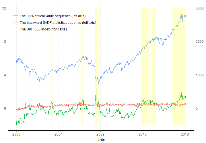
Date stamping. Fixing the endpoint r_2 and taking the sup over start dates gives a backward statistic BSADF_{r_2}; the first date at which it exceeds its critical value is the start of the bubble, the first date it falls back below is the end. A real-time monitor.
The S&P 500 through the PSY lens
Backward sup ADF sequence (blue) against its 95% critical values (red); the shaded episodes are the dates stamped as explosive. The computation is heavy because the critical values are simulated. R packages: psymonitor (Caspi) and exuber (Vasilopoulos et al.).
What to take away
A random walk has permanent shocks, a variance that grows with t, no mean to revert to. Its forecast is the last value (plus drift), with intervals that widen like \sqrt{h} forever.
Trend stationary or difference stationary is the question for every trending series. Detrend the first, difference the second; get it wrong and the long-horizon forecasts and intervals are wrong in a systematic way. The yen rewarded the model that claimed to know least.
Spurious regression. Regressions between unrelated I(1) series reject three times out of four. Allow for dynamics or difference.
Dickey-Fuller. Regress \Delta y_t on y_{t-1} (plus drift, trend and lagged differences as the data require) and compare t_\tau with simulated, not normal, critical values: about -1.95, -2.86 and -3.41 at 5%. Power is low near the null; KPSS tests the other null; read both.
In practice most macro levels are I(1); build the model on the stationary transform.
R cheat sheet
library(fpp3); library(urca)# ---- random walks and ARIMA -----------------------------------------------------------cumsum(rnorm(n)); cumsum(mu +rnorm(n)) # random walk; with driftarima.sim(n, list(order =c(p, 1, q), ar = phi, ma = theta)) # simulate an ARIMA(p,1,q)arima(y, order =c(p, 1, q)); predict(fit, n.ahead = h) # fit and forecast; base Rtsb |>model(ARIMA(y ~1+pdq(1, 1, 0) +PDQ(0, 0, 0))) # fable; "1" is a drift when d = 1tsb |>model(ARIMA(y ~1+trend() +pdq(2, 0, 0) +PDQ(0, 0, 0))) # trend-stationary alternativetsb |>model(ARIMA(y)) # d chosen by KPSS, p and q by AICc# ---- unit root tests -------------------------------------------------------------------df_t(n, R, rho =1, type ="trend") # simulate Dickey-Fuller t statistics (defined in these slides)test <-ur.df(y, type ="trend", lags =8, selectlags ="BIC") # ADF; type = "none", "drift", "trend"test@teststat; test@cval; summary(test) # statistic, critical values, the regressionur.pp(y, type ="Z-tau", model ="trend") # Phillips-Perronur.kpss(y, type ="tau") # KPSS; "mu" for constant onlytsb |>features(y, list(unitroot_kpss, unitroot_ndiffs)) # the same in fpp3tseries::adf.test(y); tseries::kpss.test(y) # alternatives with p-values
References
Additional resources
Textbooks
Diebold, F.X. (2007), Elements of Forecasting (4th ed.), the chapter “Unit Roots, Stochastic Trends, ARIMA Forecasting Models, and Smoothing”; the yen/dollar application and its data are from there.
Hamilton, J.D. (1994), Time Series Analysis, for the asymptotic theory; Pesaran, M.H. (2015), Time Series and Panel Data Econometrics; Hyndman and Athanasopoulos, FPP3, the ARIMA chapter.
Original sources
Dickey, D.A. and Fuller, W.A. (1979), JASA, 74, 427–431; Said, S.E. and Dickey, D.A. (1984), Biometrika, 71, 599–607; Phillips, P.C.B. and Perron, P. (1988), Biometrika, 75, 335–346; Kwiatkowski, Phillips, Schmidt and Shin (1992), Journal of Econometrics, 54, 159–178.
Granger, C.W.J. and Newbold, P. (1974), “Spurious Regressions in Econometrics,” Journal of Econometrics, 2, 111–120; Phillips, P.C.B. (1986), Journal of Econometrics, 33, 311–340, and (1987), Econometrica, 55, 277–301.
Nelson, C.R. and Plosser, C.I. (1982), Journal of Monetary Economics, 10, 139–162; Perron, P. (1989), Econometrica, 57, 1361–1401; Elder, J. and Kennedy, P.E. (2001), Journal of Economic Education, 32, 137–146.
Phillips, Wu and Yu (2011) and Phillips, Shi and Yu (2015), International Economic Review, 52, 201–226 and 56, 1043–1078; McCracken, M.W. and Ng, S. (2016), “FRED-MD,” Journal of Business and Economic Statistics, 34, 574–589.
Data: data/GDPC1.csv (FRED), data/2024-07-fredmd.csv (FRED-MD, July 2024 vintage), data/exchange_rates.csv (yen and DM per dollar, 1973M1 to 1996M7, Elements companion files).