Lecture 9: Assembling the Components, and Volatility Models
Zhan Gao
02 October 2026
Three components down, one to go
We have been working with y_t = T_t + S_t + C_t + \varepsilon_t: a trend, a seasonal, a cycle, and noise. The first three now each have a model, but we have fitted them one at a time.
Two things remain. First, assemble the components into one forecasting model, and see what the cycle adds to the trend-plus-seasonal forecasts of liquor sales.
Second, look harder at the noise. Every model so far ends in \varepsilon_t \sim WN(0, \sigma^2), and we have quietly read “white noise” as “independent”. Wold’s theorem needs less: only uncorrelated. The gap between the two is where volatility lives.
Today: assembling the components, and then models in which the noise has a constant unconditional variance but a conditional variance that moves: ARCH and GARCH.
Diebold, Forecasting in Economics, Business, Finance and Beyond, the chapter on assembling the components (parts 1 and 2 below) and the chapter on volatility dynamics (parts 3 to 8).
Assembling the components
The full model
Trend and seasonality were handled by regression on deterministic variables; the cycle by autoregressions. Put them in one equation by letting the regression disturbance carry the cycle:
T_t(\theta) is a trend with parameters \theta: linear, \beta_1 TIME_t; quadratic, \beta_1 TIME_t + \beta_2 TIME_t^2; and so on.
A full set of s seasonal dummies plays the role of the intercept, so none is included separately. Holiday or trading-day dummies could join them.
The disturbance follows an AR(p): the cycle. The white noise v_t is the shock that drives everything.
Any component that a particular series does not need is simply dropped. Canadian employment needed only the AR part; the retail and housing series earlier needed only a trend or a seasonal, and we ignored the cycle they very likely had.
Forecasting the full model
Write the model at T + h and project the right-hand side on \Omega_T:
Trend and seasonal variables are perfectly predictable, as before.
The twist is the disturbance. It is no longer white noise, so its future values do not project to zero. \varepsilon_{T+h,T} comes from the chain rule of the cycles lectures: \varepsilon_{T+h,T} = \phi_1 \varepsilon_{T+h-1,T} + \cdots + \phi_p \varepsilon_{T+h-p,T}, with \varepsilon_{s,T} = \varepsilon_s for s \leq T.
Operational version. Replace parameters by estimates and the unobservable disturbances by the residuals e_t:
where \hat\sigma_h^2 = \hat\sigma^2 \sum_{i=0}^{h-1} \hat\psi_i^2 is the h-step error variance of the AR disturbance, built from its moving-average weights exactly as for an autoregression.
As always, parameter estimation error is ignored in \hat\sigma_h^2. The computer does all of this; our job is to know what it is doing.
Two ways to put the cycle in
Serially correlated disturbances, as on the previous slides, or lagged dependent variables:
The two are close relatives. Multiply the disturbance model through by \Phi(L): \Phi(L) y_t = \Phi(L) T_t(\theta) + \sum_i \gamma_i \Phi(L) D_{it} + v_t. With an AR(1) disturbance and a linear trend, TIME_{t-1} = TIME_t - 1 gives
a lagged dependent variable, a trend, and white noise, but with restrictions tying the trend coefficients to \phi. The lagged-dependent-variable model leaves them free, so it is the more general of the two.
Which route?
Disturbance AR(p)
Lagged dependent variables
Estimation
nonlinear least squares or maximum likelihood
OLS
Software
arima(y, xreg = X), fable::ARIMA()
lm()
Coefficients describe
the level of y
the conditional mean of y
Generality
restricted
nests the other
In practice the difference is usually minor. What matters is to allow for the cycle somehow, so that the dynamics the trend and seasonal regressors leave behind are modeled rather than ignored. We use the disturbance version first, then check the other.
The regression-with-ARMA-disturbances view of the ARMA lecture, with trend and seasonal regressors instead of a constant.
Application: US liquor sales
Where the trend and seasonality lecture stopped
Monthly US liquor sales, 1987M1 to 2012M12 (T = 312), with 2013 and 2014 held out. The model there was a log-quadratic trend plus twelve seasonal dummies:
liquor <-tibble(Sales =scan("data/liquor_sales.csv", skip =1, quiet =TRUE)) |>mutate(Month =yearmonth(seq(as.Date("1987-01-01"), by ="month", length.out =n()))) |>as_tsibble(index = Month)lest <- liquor |>filter(year(Month) <=2012) |>mutate(TIME =row_number() /100, m =factor(month(Month), labels = month.abb)) # TIME in hundreds of monthslq <-lm(log(Sales) ~0+ TIME +I(TIME^2) + m, data = lest)round(fit_stats(lq), 4)
##      R2     SER      DW     AIC     SIC
##  0.9884  0.0444  0.6438 -6.1842 -6.0162
Trend and seasonal explain 99% of the variation in log sales, and the standard error, 0.044, is what we would expect to be off by if we forecast with trend and seasonal alone. The Durbin-Watson statistic, 0.64, says that would be leaving a lot on the table: the residuals are strongly serially correlated.
data/liquor_sales.csv, as before. TIME is measured in hundreds of months so that the quadratic term is well scaled for the numerical optimizer used below; the fit is identical to the earlier one.
The residual correlogram
corr_plot(residuals(lq), lag_max =24)
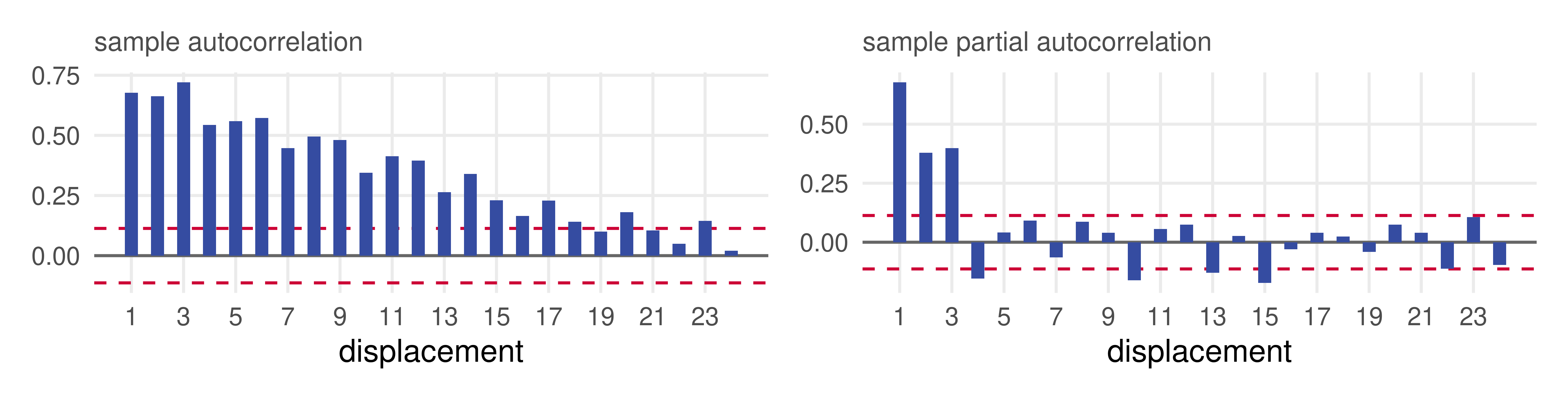
The autocorrelations are large and decay slowly, with bumps at displacements 12 and 24: the dummies have not caught all the seasonality. The partial autocorrelations are 0.68, 0.38, 0.40, then a marginal -0.15 and nothing systematic beyond: a cutoff after three. The Q statistics reject white noise everywhere. An AR(3) disturbance is the natural candidate.
Dashed lines at \pm 2/\sqrt{312} = \pm 0.11. Diebold’s correlogram of the same residuals on his 1968 to 1993 sample has the same shape.
Trend, seasonals and AR(p) disturbances
arima() with xreg estimates a regression with ARMA disturbances by maximum likelihood. Fit AR(p) disturbances for p = 0, \ldots, 4 and tabulate the usual statistics:
y <-log(lest$Sales); X <-model.matrix(lq) # the trend and seasonal regressorsdist <-lapply(0:4, function(p) arima(y, order =c(p, 0, 0), xreg = X, include.mean =FALSE))round(`rownames<-`(t(sapply(dist, ic_x, y = y)), paste0("AR(", 0:4, ")")), 4)
Allowing for the cycle cuts the standard error from 0.044 to 0.028: the forecast errors we should expect to make are 40% smaller. Both criteria fall steeply up to p = 3 and then flatten; AIC and SIC nudge toward AR(4), by 0.02 and 0.007. We go with the AR(3) the correlogram suggested. The fourth lag changes nothing of substance below.
AIC and SIC in the log-SSR form of the earlier lectures, with k counting the twelve dummies, the two trend terms and the AR coefficients. The Durbin-Watson statistic is reported for completeness; with AR disturbances it is no longer a useful test.
The AR(3) disturbance model
a3 <- dist[[4]]round(cbind(estimate =coef(a3), s.e. =sqrt(diag(a3$var.coef)))[1:5, ], 4) # AR and trend terms; dummies omitted
round(1/polyroot(c(1, -coef(a3)[1:3])), 3) # inverse AR roots
## [1] 0.942+0.000i -0.339-0.558i -0.339+0.558i
All three AR coefficients are highly significant; \hat\phi_3 = 0.40 is the largest. The trend terms barely move from the trend-only regression.
One inverse root is real and close to the unit circle, 0.94: the source of the persistence. The other two are a complex pair with modulus 0.65: a damped oscillation.
The innovation standard deviation is \hat\sigma = 0.027, half the 0.044 we had when the cycle was ignored.
Diebold finds the same configuration on his 1968 to 1993 sample: one real inverse root at .95 and a complex pair farther inside the circle.
Actual, fitted and residuals
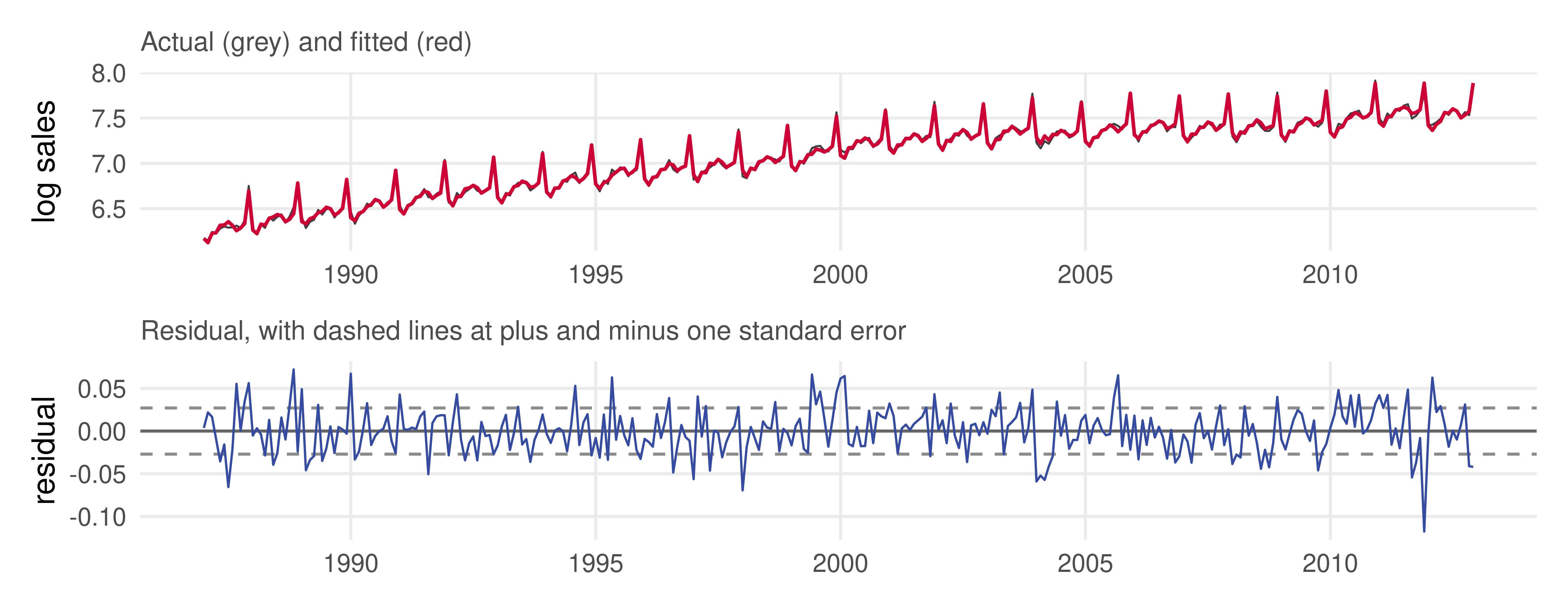
The residuals no longer trend, no longer cycle, and show no obvious seasonality; Diebold’s residual plot for his sample looks the same.
Residual correlogram
Three AR parameters were estimated, so the Q statistics are compared with \chi^2_{m-3}.
The first autocorrelations are tiny. Displacement 12 pokes above the 0.11 band (0.16): the dummies have left a trace of seasonality, and the Q statistics reject beyond displacement 10. Diebold’s correlogram shows the same pattern, and one of his exercises asks what to do about it (trading-day dummies, a seasonal AR term).
Lagged dependent variables instead
Now the other route: the same trend and seasonals, three lags of log sales on the right, OLS.
The lag coefficients, 0.26, 0.21, 0.40, are the AR(3) coefficients to two decimals, and the standard error is the same 0.028. Here the two routes are indistinguishable; the disturbance version has the advantage that its trend and seasonal coefficients describe the level of sales directly.
Diebold poses this comparison as an exercise. Three observations are lost to the lags in the OLS version; arima() keeps them by evaluating the exact likelihood.
Forecasting 2013 and 2014
Point forecasts and standard errors in logs, then exponentiate the point forecast and the interval endpoints:
new <-data.frame(TIME = (313:336) /100, m =factor(rep(month.abb, 2), levels = month.abb))Xn <-model.matrix(~0+ TIME +I(TIME^2) + m, data = new)fc <-predict(a3, n.ahead =24, newxreg = Xn) # trend + seasonal + chain-rule disturbancep0 <-predict(lq, newdata = new) # the earlier trend-plus-seasonal forecast
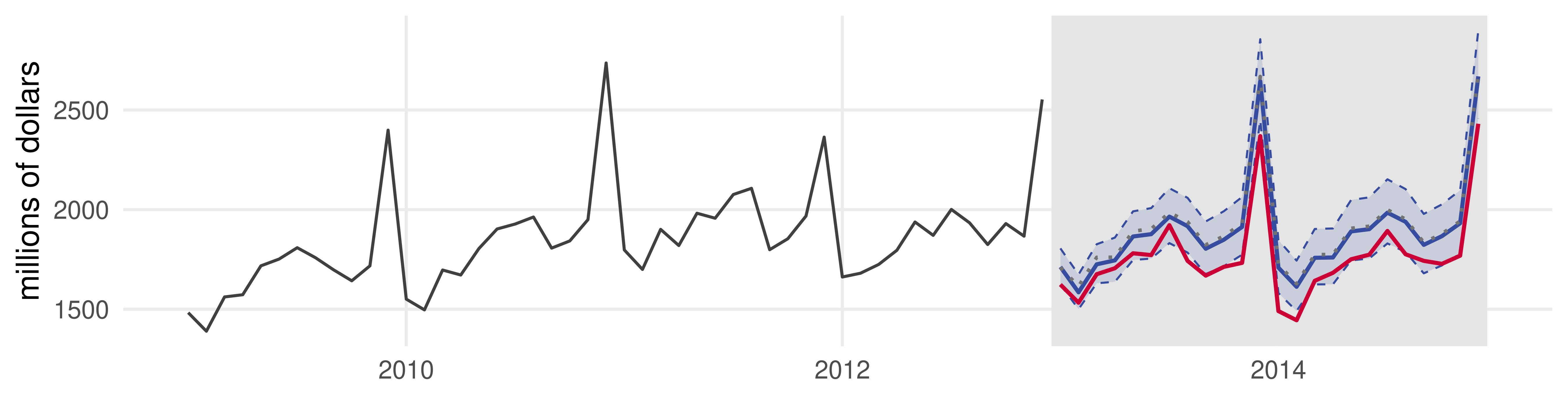
Blue: the full model with its 95% interval, from \pm 1.96 \times 0.027 at one step to \pm 1.96 \times 0.042 at 24. Dotted grey: trend and seasonal only. Red: the realization.
What did the cycle buy us?
lr <-log(lreal$y); e_ts <- lr - p0; e_ar <- lr - fc$pred # forecast errors in logsrmse <-function(e, i) sqrt(mean(e[i]^2))round(rbind(`trend + seasonal`=c(rmse(e_ts, 1:6), rmse(e_ts, 1:12), rmse(e_ts, 13:24)),`+ AR(3) disturbance`=c(rmse(e_ar, 1:6), rmse(e_ar, 1:12), rmse(e_ar, 13:24))) |>`colnames<-`(c("h = 1 to 6", "2013", "2014")), 3)
The last residuals of 2012 were negative, so the AR(3) pulls the first forecasts down by about two percent, and the short-horizon errors shrink by a fifth.
At longer horizons the correction fades, and both models over-predict by 5 to 15 percent: sales growth slowed in 2013 and 2014 more than the quadratic trend extrapolated. Out there the forecast is all trend, and the cycle cannot rescue a trend that bends.
Diebold’s 1994 forecast from the same model looked excellent. The difference is the trend, not the cycle: assembling the components fixes the near term, and the long term rests on whichever trend you chose (the subject of the unit-root lecture).
Diebold plots the same two forecasts for his sample. Realized 2013 sales were about 8 percent below the trend-plus-seasonal path.
The same in fable
ARIMA() fits regression with ARIMA errors by maximum likelihood; season() builds the dummies.
Same estimates. pdq(0:4, 0, 0:2) with stepwise = FALSE would search the disturbance order by AIC or BIC; here BIC also lands on the AR(4), AIC on an ARMA(3,2), both within a hair of the AR(3). forecast() then needs new_data with the future TIME values, and back-transforms to levels for us.
1 asks for a constant, which replaces one of the twelve dummies; the fit is the same. PDQ(0, 0, 0) switches off the seasonal ARIMA terms, which would be another way to model the leftover seasonality.
Is the noise really noise?
The residuals of the full model pass the correlogram test, more or less. White noise is uncorrelated. Is it also independent? One cheap check: the correlogram of the squared residuals.
correlogram(residuals(a3)^2, m =12)[c(1, 2, 3, 6, 12), ]
One autocorrelation pokes above the band; the rest are tiny and the Q statistic at displacement 12 does not reject. Monthly liquor sales show little sign of the pattern we are about to study. Daily stock returns are another matter entirely.
Noise with conditional variance dynamics
Strong and weak white noise
Wold’s theorem says every covariance stationary series is driven by white noise innovations, \varepsilon_t \sim WN(0, \sigma^2): zero mean, constant variance, uncorrelated. It does not say independent.
If \varepsilon_t is strong white noise, \varepsilon_t \sim \text{iid}(0, \sigma^2), the distribution of \varepsilon_t given its past is the same as its unconditional distribution, by definition of independence. Then \sigma^2 is both the unconditional and the conditional variance.
If \varepsilon_t is only weak white noise, uncorrelated but dependent, the two distributions differ. Write \varepsilon_t \sim (0, \sigma^2) unconditionally and
The conditional variance \sigma_t^2 evolves as the information set evolves: conditional heteroskedasticity, or time-varying volatility. So far we have assumed strong white noise, sometimes explicitly and sometimes without noticing.
Other features of the conditional distribution, such as skewness, could move as well. Variance dynamics are by far the most important in practice, so we attribute all movement in the conditional distribution to \sigma_t^2.
Why care?
Finance. Markets are sometimes tranquil and sometimes turbulent. Risk management, asset allocation and option pricing all need the volatility now, not its long-run average. Modeling and forecasting it is a central part of financial econometrics.
Forecasting, everywhere. Interval and density forecasts rest on the forecast error variance. If volatility moves, correct intervals must widen and narrow with it: the \pm 1.96\, \sigma_h bands of the cycles lectures depend on h only, and nothing in those models could make them depend on the state of the world at T.
Models built for the first problem solve the second. The running example is a series with no trend, no seasonal and hardly any cycle, where volatility is the whole story.
Daily stock returns
r <-100*scan("data/nyse_returns.csv", skip =1, quiet =TRUE) # daily NYSE returns, in percenty <- r[1:3461]; hold <- r[3462:3531] # estimation sample; 70 days held outggplot(data.frame(t =seq_along(y), r = y), aes(t, r)) +geom_hline(yintercept =0, colour ="grey40") +geom_line(colour = smu_blue, linewidth =0.3) + yr_axis +labs(x =NULL, y ="return, %")
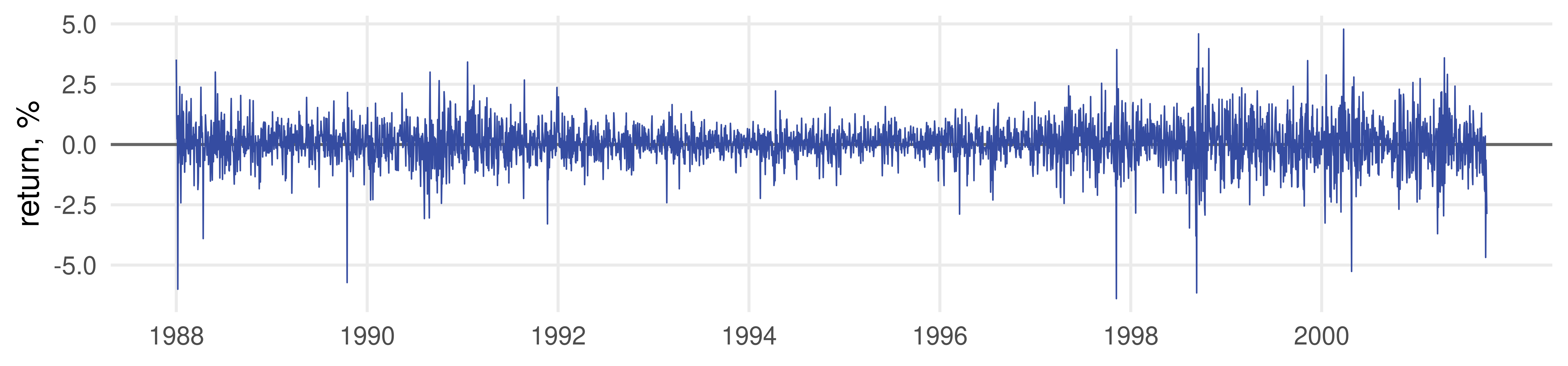
Daily returns on the NYSE index, January 1988 to December 2001. Tranquil stretches and turbulent ones: the amplitude of the returns is serially correlated even if the returns themselves are not. That is volatility clustering, and it is what we model.
The file carries no dates; the axis labels assume 252 trading days a year.
The general linear process with iid innovations
Recall y_t = B(L)\varepsilon_t = \sum_{i \geq 0} b_i \varepsilon_{t-i} with \varepsilon_t \sim \text{iid}(0, \sigma^2). Its unconditional mean and variance are constant, and its conditional mean moves:
Different from the unconditional variance, yes, but it depends on h only. The conditional variance is not allowed to adapt to readily available information.
The ability to capture conditional mean dynamics is the source of the general linear process’s power. We now let the innovation be weak white noise with a particular dependence structure, so that conditional variance dynamics are captured too.
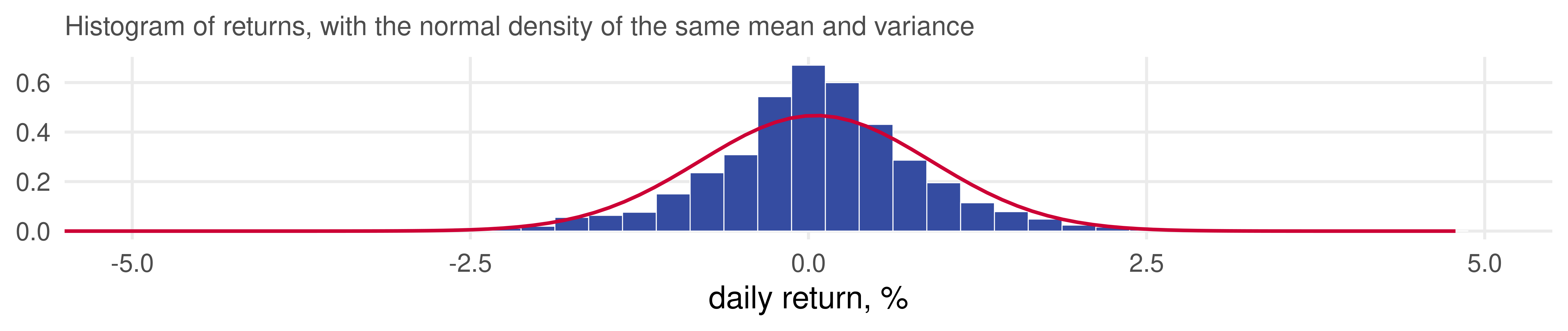
##     mean       sd skewness kurtosis
##    0.052    0.854   -0.505    8.530
The mean return is slightly positive. The distribution is nearly symmetric but far more peaked and fat-tailed than the normal: kurtosis 8.5 against 3, and the Jarque-Bera statistic is in the thousands.
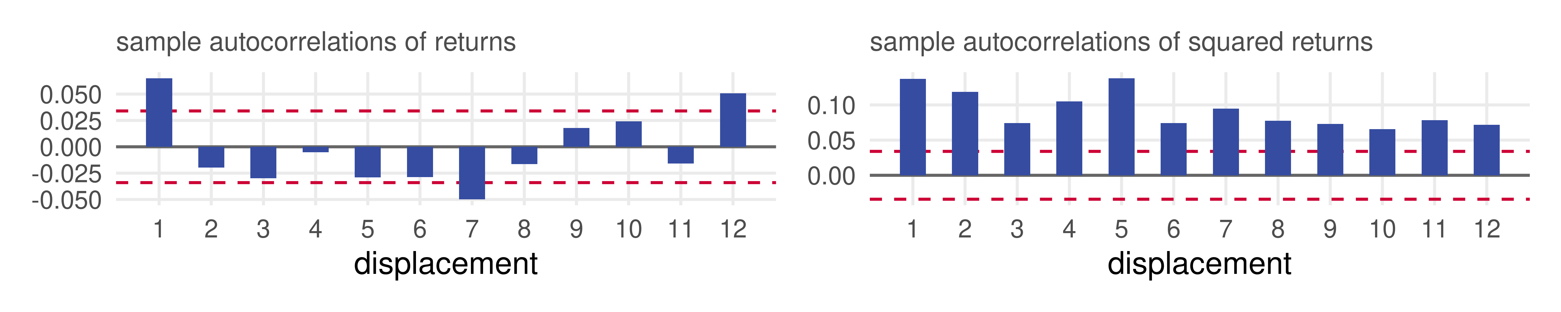
The returns’ own autocorrelations are tiny (\hat\rho(1) = 0.07, band \pm 0.03); Q(12) = 47 rejects white noise, but the dynamics are weak and we proceed as if returns were white noise.
Volatility clustering, seen
Large changes are followed by large changes, small by small, of either sign. Every autocorrelation of the squares is positive and far outside the band (Q(12) = 381): volatility is persistent even though returns are not.
The ARCH process
Autoregressive conditional heteroskedasticity
Keep y_t = B(L)\varepsilon_t, but parameterize the innovation through its conditional density:
Zero conditional mean, and a conditional variance that depends linearly on the p most recent squared innovations. \varepsilon_t is an ARCH(p) process (Engle, 1982).
\varepsilon_t is serially uncorrelated but not independent: today’s variance depends on the history of \varepsilon. The conditions keep both variances positive and finite and y_t covariance stationary.
Large \varepsilon^2’s in the recent past produce a large \sigma_t^2 today, hence a large \varepsilon_t^2 today is likely: clustering. ARCH approximates volatility dynamics autoregressively, hence the name. ARCH is to the conditional variance what AR is to the conditional mean.
Moments of an ARCH process
Unconditional.E(\varepsilon_t) = 0. For the variance, take expectations of the variance equation and use that E(\varepsilon_t^2) = \sigma^2 is the same at every date under stationarity:
Fixed, as covariance stationarity requires. The particular formula matters less than that fact.
Conditional.E(\varepsilon_t \mid \Omega_{t-1}) = 0 by construction, and \operatorname{var}(\varepsilon_t \mid \Omega_{t-1}) = \omega + \gamma(L)\varepsilon_t^2: time-varying.
Moving to y_t = B(L)\varepsilon_t. Unconditional mean and variance constant; conditional mean \sum_{i \geq 1} b_i \varepsilon_{t-i} and conditional variance \omega + \gamma(L)\varepsilon_t^2 both move with \Omega_{t-1}. Conditional mean and variance dynamics are now treated symmetrically.
Two uses. As a model for the disturbance of a broader model, as above. Or, when there are no conditional mean dynamics worth modeling, for an observed series directly. Asset returns are the leading case: negligible mean dynamics, strong variance dynamics. We call the series a “return”.
ARCH(1), simulated
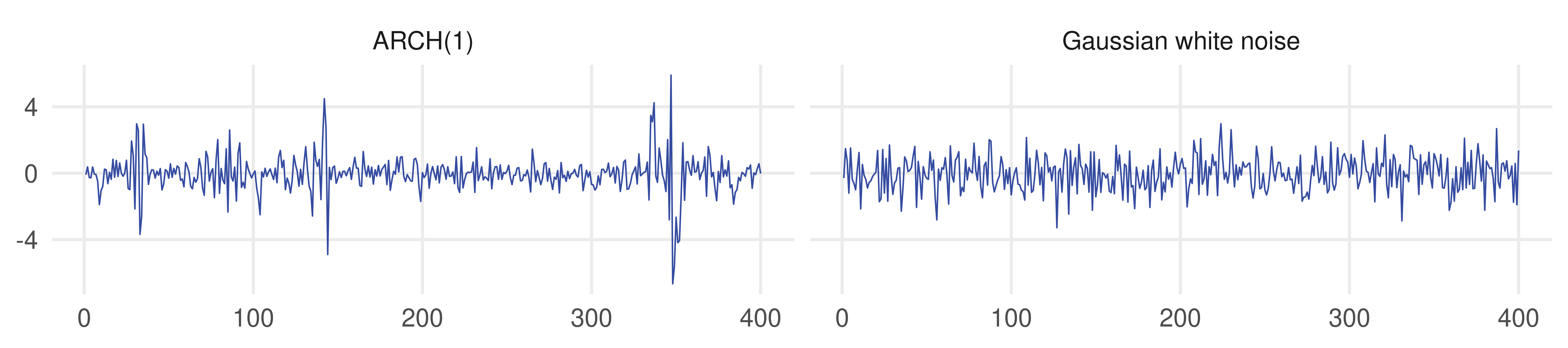
\sigma_t^2 = 0.2 + 0.8\, \varepsilon_{t-1}^2 against Gaussian white noise, both with unconditional variance 1.
set.seed(8); n <-400; v <-rnorm(n); e <-numeric(n); s2 <-numeric(n); s2[1] <-1; e[1] <- v[1]for (t in2:n) { s2[t] <-0.2+0.8* e[t -1]^2; e[t] <-sqrt(s2[t]) * v[t] } # e_t = sigma_t * v_td <-data.frame(t =rep(1:n, 2), series =rep(c("ARCH(1)", "Gaussian white noise"), each = n),e =c(e, rnorm(n)))ggplot(d, aes(t, e)) +geom_line(colour = smu_blue, linewidth =0.3) +facet_wrap(~ series) +labs(x =NULL, y =NULL)
Same variance, different texture: the ARCH series has quiet stretches and bursts, and its extremes are larger. The construction \varepsilon_t = \sigma_t v_t with v_t \sim \text{iid}\, N(0,1) is how every ARCH-type process is simulated, and how it is checked after estimation.
ARCH(1), simulated: the correlograms
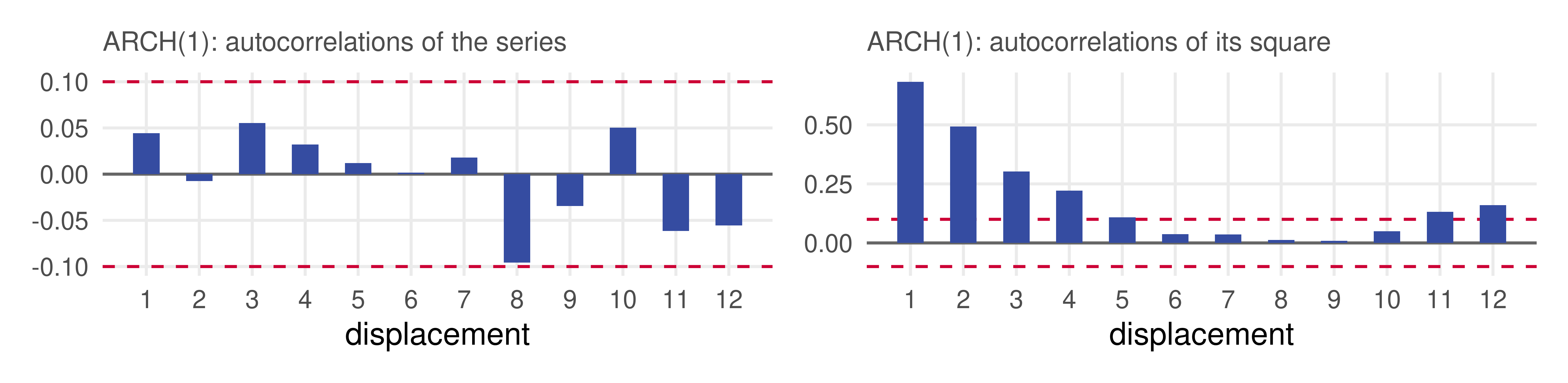
The autocorrelations of the series are zero: ARCH is white noise. Those of its square decay like 0.8^\tau, because \varepsilon_t^2 = \omega + \gamma\, \varepsilon_{t-1}^2 + \nu_t with \nu_t = \varepsilon_t^2 - \sigma_t^2 is an AR(1) in the squares, as the next section shows. Dependence without correlation: the correlogram of the squares is where it shows up.
Testing for ARCH effects
Engle’s LM test: regress the squared residuals of the conditional mean model on q of their own lags, and compare T R^2 with \chi^2_q. Under the null of no ARCH all q slopes are zero.
arch_lm <-function(e, q) { # e: residuals from the conditional mean model d <-data.frame(e2 = e^2); for (i in1:q) d[[paste0("L", i)]] <- dplyr::lag(d$e2, i) fit <-lm(e2 ~ ., data = d); LM <- (nrow(d) - q) *summary(fit)$r.squaredc(LM = LM, p =pchisq(LM, q, lower.tail =FALSE))}arch_lm(y -mean(y), q =5)
##           LM            p
## 1.794505e+02 7.011292e-37
The null is rejected without any doubt. The correlogram of squared residuals, as on the earlier slide, is the graphical version of the same evidence.
Order of operations matters: model the conditional mean first, then look at the squares of what is left. Neglected serial correlation in the mean also produces serial correlation in \varepsilon_t^2, and would be mistaken for volatility dynamics. Here the mean model is just a constant.
The GARCH process
Generalized ARCH
Bollerslev’s (1986) GARCH(p,q) adds lagged conditional variances to the variance equation. The pure GARCH process, with y_t = \varepsilon_t, is
The workhorse is GARCH(1,1): \sigma_t^2 = \omega + \alpha\, \varepsilon_{t-1}^2 + \beta\, \sigma_{t-1}^2. Today’s variance is a weighted average of a constant, yesterday’s squared shock, and yesterday’s variance.
\beta(L) = 0 gives back ARCH(p). \alpha(L) = \beta(L) = 0 gives iid Gaussian noise with variance \omega: white noise is a special, highly restrictive case of GARCH, not the other way around.
GARCH is to ARCH (for the variance) as ARMA is to AR (for the mean): the same parsimony argument.
“Pure” means no conditional mean dynamics; adding them, as in y_t = B(L)\varepsilon_t, clutters the notation and changes nothing below. For a return, “pure” is usually the right model anyway.
Current volatility is an exponentially weighted moving average of past squared shocks.
Compare exponential smoothing of \varepsilon_t^2, \bar\varepsilon_t^2 = \lambda \varepsilon_t^2 + (1 - \lambda)\bar\varepsilon_{t-1}^2, which also puts weights \lambda(1-\lambda)^j on past squares. GARCH(1,1) is that smoother with \omega added and the smoothing parameter estimated rather than set by convention. RiskMetrics’ \lambda = 0.06 for daily data is a GARCH(1,1) with \alpha = 0.06, \beta = 0.94, \omega = 0.
Unconditional moments: stationarity and fat tails
The same trick as for ARCH, with E(\varepsilon_t^2) = E(\sigma_t^2) = \sigma^2 at every date:
The unconditional variance is fixed; the conditional variance is itself a serially correlated time series.
Higher moments. Even with a conditionally normal innovation, the unconditional distribution is symmetric but leptokurtic. For GARCH(1,1), when it is finite,
Clusters of low and high volatility put observations in the center and in the tails more often than a fixed-variance normal would. Asset returns look exactly like that, and GARCH was not built to explain it: the fat tails come free.
Bollerslev (1986); with \alpha = 0.06 and \beta = 0.93 the kurtosis is about 4.7. Sums of GARCH processes obey a central limit theorem, so weekly and monthly returns are closer to normal than daily ones, which is also a fact.
Squared shocks follow an ARMA process
Define \nu_t = \varepsilon_t^2 - \sigma_t^2: the surprise in the squared shock, with E(\nu_t \mid \Omega_{t-1}) = 0, so \nu_t is white noise. Add and subtract \beta(L)\varepsilon_t^2 in the variance equation:
The squared innovation is an ARMA(\max(p,q), q) process with innovation \nu_t. For GARCH(1,1), an ARMA(1,1) whose autoregressive coefficient is \alpha + \beta.
Hence the slowly decaying, all-positive correlogram of squared returns: with \alpha + \beta near one the autocorrelations of \varepsilon_t^2 die out very slowly.
\varepsilon_t^2 is an unbiased but noisy proxy for \sigma_t^2; the GARCH recursion is the smoothing that reconciles the two. An AR fitted directly to \varepsilon_t^2 is a crude first pass at the same idea.
\nu_t \in [-\sigma_t^2, \infty): far from normal, but uncorrelated with its own past.
Forecasting the conditional variance
Everything that determines \sigma_{t+1}^2 is dated t or earlier, so the one-step forecast is known exactly: \sigma^2_{t+1,t} = \omega + \alpha \varepsilon_t^2 + \beta \sigma_t^2. For h \geq 2, take conditional expectations of the variance equation at t+h, using E(\varepsilon_{t+h-1}^2 \mid \Omega_t) = E(\sigma_{t+h-1}^2 \mid \Omega_t):
The h-step forecast is the one-step forecast pulled toward the unconditional variance at the geometric rate \alpha + \beta; a volatility shock has half-life \ln(0.5) / \ln(\alpha + \beta).
As h \to \infty the forecast reaches \bar\sigma^2: today’s turbulence says nothing about the distant future, just as today’s level tells an AR nothing about the distant mean. For finite h it depends on \Omega_t, which is what we wanted.
For GARCH(p,q) replace \alpha + \beta by \alpha(1) + \beta(1). Feasible forecasts \hat\sigma^2_{t+h,t} insert the estimates.
Interval forecasts that breathe
With constant volatility the 95% interval for y_{t+h} was y_{t+h,t} \pm 1.96\, \sigma_h, where \sigma_h is the h-step forecast error standard deviation, the same at every date. With volatility dynamics,
y_{t+h,t} \;\pm\; 1.96\, \sigma_{t+h,t} .
When volatility is low the interval is tight; when it is high, wide. The constant-volatility interval is correct on average but wrong at almost every date; the conditional interval is correct at all dates. The same holds for the density forecast N(y_{t+h,t}, \sigma^2_{t+h,t}).
For a pure GARCH return the point forecast is boring, E(\varepsilon_{t+h} \mid \Omega_t) = 0 (or the mean), and the forecast error is the return itself. All the action is in the interval. In many financial applications the volatility forecast \sigma^2_{t+h,t} is itself the object of interest.
Under asymmetric loss even point forecasts change: the optimal predictor is the conditional mean shifted by an amount that grows with \sigma_{t+h,t} (Christoffersen and Diebold, 1997).
Estimation and diagnostics
Maximum likelihood
Conditional normality gives the density of each observation given its past, and the joint density is the product of these conditional densities:
with \theta = (\omega, \alpha, \beta) and \sigma_t^2(\theta) computed recursively from the data and a starting value.
No closed form: the likelihood is maximized numerically. As with any numerical optimization, starting values and convergence criteria need care (local maxima exist).
The likelihood penalizes a large \varepsilon_t^2 less when \sigma_t^2 is large: the fit “explains” a burst by a high conditional variance, and pays through the \ln \sigma_t^2 term for calling every period a burst.
If the conditional distribution is not normal, the Gaussian estimator is still consistent (quasi-maximum likelihood, Bollerslev and Wooldridge, 1992); only the standard errors need a robust formula.
With a conditional mean model, \varepsilon_t is replaced by y_t - \mu_t(\theta) and the mean parameters are estimated jointly.
GARCH(1,1) in ten lines
The variance recursion and the log likelihood are all there is. Start the recursion at the sample variance, demean the returns, and hand the function to optim():
garch11_nll <-function(par, e) { # par = (omega, alpha, beta); e = demeaned returns om <- par[1]; al <- par[2]; be <- par[3]; n <-length(e) s2 <-numeric(n); s2[1] <-var(e)for (t in2:n) s2[t] <- om + al * e[t -1]^2+ be * s2[t -1]-sum(dnorm(e, 0, sqrt(s2), log =TRUE)) # minus the Gaussian log likelihood}e <- y -mean(y)opt <-optim(c(0.05, 0.05, 0.9), garch11_nll, e = e, method ="L-BFGS-B",lower =1e-6, upper =c(5, 1, 1), hessian =TRUE)round(rbind(estimate = opt$par, s.e. =sqrt(diag(solve(opt$hessian)))), 4)
\hat\omega = 0.009, \hat\alpha = 0.064, \hat\beta = 0.926. The standard errors come from the inverse Hessian at the optimum, the usual maximum likelihood recipe.
The same with rugarch
ugarchspec() describes the model, ugarchfit() estimates it, with the mean estimated jointly:
All coefficients highly significant. The “ARCH coefficient” \alpha and the “GARCH coefficient” \beta sum to 0.99 with \beta far larger than \alpha, as is typical of asset returns: a volatility shock has a half-life of seventy trading days. The unconditional standard deviation is 0.94 percent a day.
Diebold’s own GARCH(1,1) estimates on these data: \hat\alpha + \hat\beta = .987 and an unconditional standard deviation of .009 in decimal returns.
Diagnostics: standardized residuals
Since \varepsilon_t = \sigma_t v_t with v_t \sim \text{iid}\, N(0,1), the standardized residuals\hat v_t = \varepsilon_t / \hat\sigma_t of an adequate model are iid, and their squares show no autocorrelation:
z <-as.numeric(residuals(g11, standardize =TRUE))correlogram(z^2, m =12, dof =2)[c(1, 2, 3, 6, 12), ]
Every autocorrelation is inside the band and Q is nowhere near rejection: the GARCH(1,1) has captured the volatility dynamics. But the standardized residuals still have kurtosis 8: the conditional normality assumption is wrong. The estimates survive (quasi-maximum likelihood); for density forecasts, move to Student’s t innovations.
Q against \chi^2_{m-k}, k the number of GARCH parameters (Bollerslev and Mikkelsen, 1996).
Application: NYSE stock market volatility
A crude first pass: an AR(5) on squared returns
Squared returns proxy the conditional variance, so why not regress r_t^2 on its own lags?
d <-data.frame(r2 = y^2); for (i in1:5) d[[paste0("L", i)]] <- dplyr::lag(d$r2, i)ar5 <-lm(r2 ~ ., data = d)round(summary(ar5)$coefficients, 4); round(summary(ar5)$r.squared, 3)
The lags are mostly significant, even the fifth, yet R^2 = 0.05: the squared return is a very noisy proxy, as \nu_t = \varepsilon_t^2 - \sigma_t^2 reminded us. Diebold reports the same regression.
ARCH(5)
Second pass: an ARCH(5) for the returns, by maximum likelihood.
z5 <-as.numeric(residuals(a5, standardize =TRUE))Box.test(z5^2, lag =12, type ="Ljung-Box", fitdf =5)$p.value # Q(12) on squared standardized residuals
## [1] 0.02430578
The lagged squared returns are significant even at long lags, yet the squared standardized residuals still reject white noise: the ARCH(5) misses part of the dynamics. GARCH supplies the longer lags with two parameters.
AIC per observation is 2.40 for the ARCH(5) and 2.35 for the GARCH(1,1); Diebold’s estimates agree.
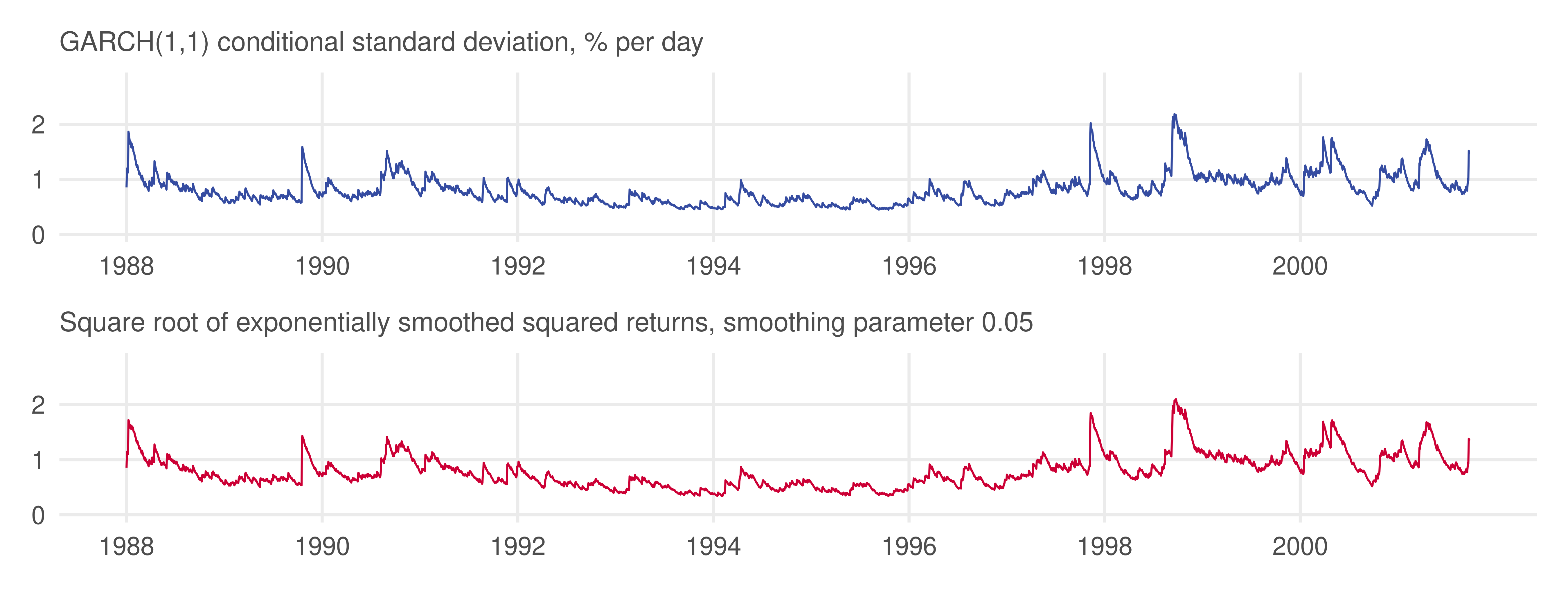
The estimated conditional standard deviation
Volatility fluctuates a great deal and is highly persistent: calm in the mid-1990s, bursts in 1997 and 1998. The two estimates behave similarly but not identically; the GARCH smoothing parameter is estimated by maximum likelihood, the exponential smoothing one set by convention.
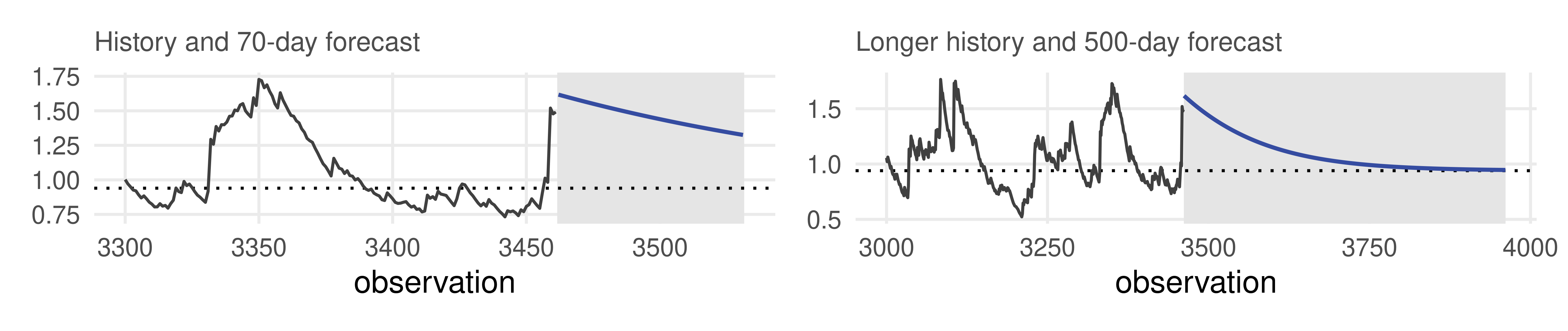
Forecasting volatility out of sample
Estimated on the first 3461 days; forecast the conditional standard deviation for the 70 held-out days and beyond:
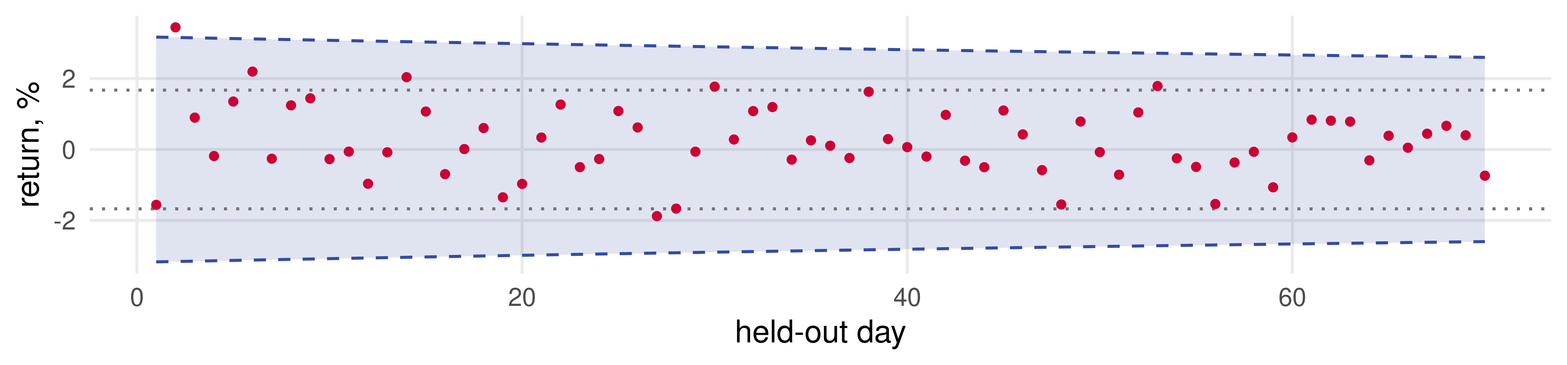
Red points: realized returns. Blue: the GARCH interval, wide after the burst and narrowing; dotted grey: the constant interval. Seven of the 70 returns fall outside the constant bands (90% coverage); one falls outside the GARCH bands. Volatility was high, and the model knew it.
Extensions
Asymmetric response: bad news is louder
In GARCH only the square of yesterday’s return matters, so its sign is irrelevant. For stocks, negative returns raise volatility more than positive ones of the same size: the leverage effect. Two fixes, both in the GARCH(1,1) setting:
Threshold GARCH (TGARCH, or GJR), with D_{t-1} = 1 if \varepsilon_{t-1} < 0 and 0 otherwise:
The size of the news enters through |\varepsilon_{t-1}/\sigma_{t-1}|, its sign through \varepsilon_{t-1}/\sigma_{t-1}.
TGARCH: Glosten, Jagannathan and Runkle (1993); EGARCH: Nelson (1991). The name “leverage”: a fall in equity value raises a firm’s debt-to-equity ratio, hence its leverage and its risk.
\hat\gamma = 0.09 with a t statistic near 5: a negative return raises next day’s variance by \hat\alpha + \hat\gamma = 0.12 times its square, a positive return by only 0.03. The log likelihood rises by 21 for one extra parameter. Asymmetry is real in stock returns, and the symmetric GARCH(1,1) is a first approximation.
Replacing "gjrGARCH" by "eGARCH" fits the exponential version, which raises the likelihood further; Diebold poses the comparison as an exercise.
All of these can be mixed, and rugarch has every one of them. On the NYSE data the t model estimates d \approx 5 degrees of freedom and raises the log likelihood by 170: the fat conditional tails matter more than any other extension.
GARCH-M: Engle, Lilien and Robins (1987); component GARCH: Engle and Lee (1999); t-GARCH: Bollerslev (1987).
Where volatility modeling went next
Multivariate GARCH. A portfolio needs conditional covariances too. The general model has far too many parameters for more than a handful of assets; parsimonious versions (constant and dynamic conditional correlation, factor GARCH) are the practical tools.
Realized volatility. With intraday data, the sum of squared five-minute returns over a day measures that day’s variance almost without error. Volatility becomes an observed series, to be forecast with the ordinary tools of this course (Andersen, Bollerslev, Diebold and Labys, 2003). The Risk Lab at Chicago Booth posts daily realized volatilities for thousands of assets.
Predictability. Returns are nearly unpredictable; their volatility is highly predictable. Economic variables that fail to forecast returns often help forecast volatility (Christiansen, Schmeling and Schrimpf, 2012). For a forecaster, the second moment is the better target.
What to take away
Assembling. Trend and seasonals enter as regressors, the cycle as an AR disturbance or as lagged dependent variables; both routes give nearly the same forecasts. Forecast the deterministic parts exactly and the disturbance by the chain rule. For liquor sales the cycle cut the one-step error standard deviation by 40 percent and fixed the near term; the long term is the trend’s responsibility.
Weak white noise. Uncorrelated need not mean independent. Conditional variance dynamics leave the unconditional variance constant but make \sigma_t^2 move with the information set.
ARCH and GARCH.\sigma_t^2 = \omega + \alpha \varepsilon_{t-1}^2 + \beta \sigma_{t-1}^2 is an exponentially weighted average of past squared shocks; \varepsilon_t^2 follows an ARMA; the unconditional distribution is fat-tailed for free. GARCH is to ARCH as ARMA is to AR.
Forecasts.\sigma^2_{t+h,t} reverts to \omega/(1 - \alpha - \beta) at rate \alpha + \beta. Intervals y_{t+h,t} \pm 1.96\, \sigma_{t+h,t} widen and narrow with the state of the market.
Practice. Estimate by maximum likelihood, check the correlogram of squared standardized residuals, expect \alpha + \beta near one, and consider asymmetry and t innovations for stocks.
R cheat sheet
library(rugarch); library(fpp3)# ---- assembling the components ------------------------------------------------------arima(y, order =c(p, 0, 0), xreg = X) # regression on X with AR(p) disturbances, MLpredict(fit, n.ahead = h, newxreg = Xn) # point forecasts and standard errorstsb |>model(ARIMA(log(y) ~1+ TIME +I(TIME^2) +season() +pdq(p, 0, 0) +PDQ(0, 0, 0))) # fablelm(y ~0+ TIME +I(TIME^2) + m + L1 + L2 + L3) # lagged-dependent-variable version, OLS# ---- volatility: diagnostics ---------------------------------------------------------Box.test(y^2, lag =12, type ="Ljung-Box") # Q test on squared returnsarch_lm(y -mean(y), q =5) # Engle's LM test (defined in these slides)correlogram(z^2, m =12, dof = k) # squared standardized residuals, chi-square(m - k)# ---- volatility: estimation and forecasting ------------------------------------------spec <-ugarchspec(variance.model =list(model ="sGARCH", garchOrder =c(1, 1)), # or "gjrGARCH", "eGARCH"mean.model =list(armaOrder =c(0, 0)), distribution.model ="norm") # or "std"fit <-ugarchfit(spec, y); fit@fit$matcoef # estimates, standard errors, t statisticssigma(fit); residuals(fit, standardize =TRUE) # conditional sd path; standardized residualspersistence(fit); halflife(fit); uncvariance(fit) # alpha + beta, half-life, unconditional variancesigma(ugarchforecast(fit, n.ahead = h)) # h-step conditional sd forecastsoptim(start, garch11_nll, e = e, method ="L-BFGS-B", lower =1e-6) # by hand (garch11_nll defined in these slides)
References
Additional resources
Textbooks
Diebold, F.X. Forecasting in Economics, Business, Finance and Beyond, the chapters on volatility dynamics and on assembling the components. The liquor and NYSE data come from the book’s companion files.
Pesaran, M.H. (2015), Time Series and Panel Data Econometrics, for a fuller treatment of ARCH and GARCH.
Engle, R.F. (1982), “Autoregressive Conditional Heteroscedasticity with Estimates of the Variance of United Kingdom Inflation,” Econometrica, 50, 987–1007. Bollerslev, T. (1986), “Generalized Autoregressive Conditional Heteroskedasticity,” Journal of Econometrics, 31, 307–327.
Glosten, L.R., Jagannathan, R. and Runkle, D.E. (1993), Journal of Finance, 48, 1779–1801; Nelson, D.B. (1991), Econometrica, 59, 347–370; Engle, R.F., Lilien, D.M. and Robins, R.P. (1987), Econometrica, 55, 391–407; Engle, R.F. and Lee, G.G.J. (1999), in Cointegration, Causality and Forecasting, Oxford.
Bollerslev, T. and Wooldridge, J.M. (1992), Econometric Reviews, 11, 143–172. Christoffersen, P.F. and Diebold, F.X. (1997), Econometric Theory, 13, 808–817.
Andersen, T.G., Bollerslev, T., Diebold, F.X. and Labys, P. (2003), “Modeling and Forecasting Realized Volatility,” Econometrica, 71, 579–625. Christiansen, C., Schmeling, M. and Schrimpf, A. (2012), Journal of Applied Econometrics, 27, 956–977.
Software: Ghalanos, A., rugarch: Univariate GARCH models, R package. Alternatives: fGarch::garchFit(), tseries::garch().
Data: data/liquor_sales.csv (monthly US liquor sales, 1987M1 to 2014M12), data/nyse_returns.csv (daily NYSE returns, 1988 to 2001, 3531 observations), both from the companion files.