Last time we fit an AR(2) to Canadian employment and forecast it with Wold’s chain rule. It worked. Two questions were left open.
Why is an autoregression the right kind of model for a covariance stationary series? And would a different approximation, a moving average or a mixed model, do better?
Wold’s theorem answers the first: every covariance stationary series is an infinite moving average of white noise. MA, AR and ARMA models are three parsimonious approximations to that representation.
Today: the theorem and its approximations, forecasting from the moving-average side and from the autoregressive side, estimation (and the small-sample bias of OLS), and the employment data fitted three ways.
Diebold, Forecasting in Economics, Business, Finance and Beyond, Chapter 7, point forecasts only (interval and density forecasts are its Sections 7.3.3 and 7.4.3). Section 7 also draws on Pesaran (2015), Chapter 14.
The Wold representation and its approximation
Wold’s theorem
Many different dynamic patterns are consistent with covariance stationarity. Knowing only that a series is stationary, what should we fit to what is left after the trend and the seasonal? The theorem previewed last week says what the model must look like.
Theorem (Wold, 1938). Let y_t be any zero-mean covariance stationary process with no deterministic components. Then
The correct “model” for any covariance stationary series is some infinite distributed lag of white noise, the Wold representation.
The \varepsilon_t are the innovations: the one-step-ahead errors of the best linear forecast, the part of y_t that is linearly unpredictable from its own past. Uncorrelated, not necessarily independent.
Zero mean is no restriction. Whenever you see y_t, read y_t - \mu.
The general linear process
The Wold form, y_t = \sum_{i\ge 0} b_i \varepsilon_{t-i}, is called the general linear process: general because every stationary series can be written this way, linear because y_t is linear in its innovations. Its moments follow in two lines.
Unconditional.E(y_t) = \sum_i b_i\, E(\varepsilon_{t-i}) = 0 and \operatorname{var}(y_t) = \sum_i b_i^2 \operatorname{var}(\varepsilon_{t-i}) = \sigma^2 \sum_i b_i^2, finite by the square summability.
Conditional on \Omega_{t-1} = \{\varepsilon_{t-1}, \varepsilon_{t-2}, \ldots\}:
The key insight, again: the unconditional mean is a constant, as stationarity requires, while the conditional mean moves with the information set. Capturing those conditional-mean dynamics is the forecaster’s whole job.
The conditional variance is constant here, which will be extended by the volatility models.
Approximating the Wold representation
We never pretend the fitted model is true; we approximate a more complex reality. The representation has infinitely many coefficients, but an infinite lag polynomial need not have infinitely many free parameters. Suppose
Such a B(L) is a rational polynomial; it has only p + q parameters, however many terms its expansion has. If B(L) is only approximately rational, a rational distributed lag still approximates it well while economizing on parameters.
Model
B(L)
Free parameters
Signature
MA(q)
\Theta(L)
q
numerator only
AR(p)
1/\Phi(L)
p
denominator only
ARMA(p,q)
\Theta(L)/\Phi(L)
p+q
both
Each family has its own autocorrelation signature. We derive them assuming the model is true, then read sample correlograms and AIC/SIC to choose among candidates.
Moving average models
The MA(1) process
The finite-order moving average is the most direct approximation to the Wold form: truncate the infinite moving average. The first-order moving average, MA(1), is
A regression with nothing but current and lagged unobservable disturbances on the right.
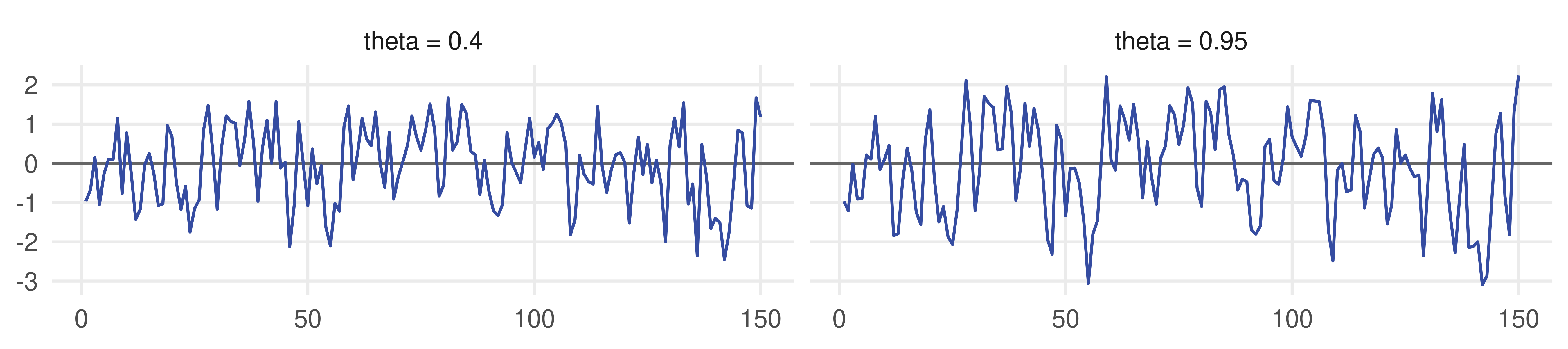
set.seed(3); e <-rnorm(150) # one shock sequence for bothma1 <-function(theta) e + theta *c(0, head(e, -1))d <-data.frame(t =rep(1:150, 2), theta =rep(c("theta = 0.4", "theta = 0.95"), each =150),y =c(ma1(0.4), ma1(0.95)))ggplot(d, aes(t, y)) +geom_hline(yintercept =0, colour ="grey40") +geom_line(colour = smu_blue) +facet_wrap(~ theta) +labs(x =NULL, y =NULL)
You might expect \theta = 0.95 to be much more persistent than \theta = 0.4. It is not. Only one lag of the shock enters, so the memory is one period, whatever the parameter.
Moments of the MA(1)
Unconditional.E(y_t) = E(\varepsilon_t) + \theta E(\varepsilon_{t-1}) = 0 and \operatorname{var}(y_t) = \sigma^2 + \theta^2 \sigma^2 = \sigma^2(1 + \theta^2). For fixed \sigma, a larger |\theta| means a larger variance: that is why the \theta = 0.95 realization swings a little wider, not because it is more persistent.
Conditional on \Omega_{t-1} = \{\varepsilon_{t-1}, \varepsilon_{t-2}, \ldots\}:
The conditional mean adapts to the information set, but only through the most recent shock. Shocks two or more periods old have no effect on today’s conditional expectation: the one-period memory again, now in the moments.
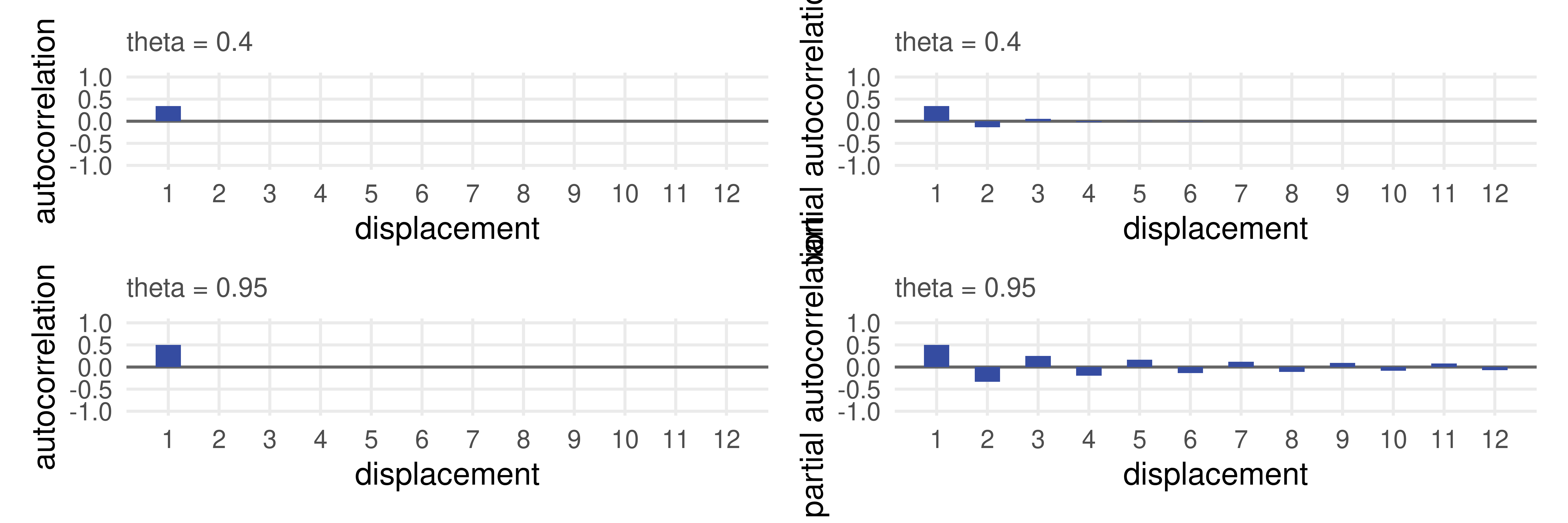
White noise kills every product of shocks at different dates. At \tau = 0 the first and last terms survive, \gamma(0) = \sigma^2(1 + \theta^2); at \tau = 1 only the third, \gamma(1) = \theta \sigma^2; at \tau \geq 2 nothing. Hence
A sharp cutoff at displacement 1, the order of the process. For \theta = 0.4, \rho(1) = 0.34; for \theta = 0.95, \rho(1) = 0.50. And \rho(1) can never exceed 1/2: no MA(1) is strongly autocorrelated.
Diebold, Chapter 7, Exercise 2. The bound follows from (1 - |\theta|)^2 \geq 0.
Invertibility
The MA(1) is covariance stationary for any\theta: constant mean, finite constant variance, autocorrelations depending only on the displacement. A second property needs a condition. Solve for the innovation and substitute backward:
This is the autoregressive representation, \frac{1}{1+\theta L}\, y_t = \varepsilon_t: the current value in terms of a current shock and lagged observables. The back substitution raises \theta to ever higher powers, so it converges only if |\theta| < 1. Then the MA(1) is invertible.
Equivalently, the root of 1 + \theta L = 0 is L = -1/\theta, and invertibility says its inverse, -\theta, lies inside the unit circle. The inverse-root form generalizes to higher orders.
Why care? A model used for forecasting must link the present to the observed past, so that we can extrapolate. Moving averages seem not to qualify, but invertible ones do, through their AR representation. We therefore restrict attention to invertible processes.
The MA(1) partial autocorrelation function
From the infinite autoregressive representation, the PACF decays gradually rather than cutting off. With \theta > 0 the AR coefficients \theta, -\theta^2, \theta^3, \ldots alternate in sign, so the decay is a damped oscillation; it is slower for \theta = 0.95.
Diebold’s Figures 7.2 to 7.5. The partial autocorrelations are not the AR(\infty) coefficients themselves; they are the last coefficients of successively longer autoregressions.
Everything parallels the MA(1), so we state the properties without grinding through the algebra.
Stationary for any parameter values.
Invertible if and only if the inverses of all q roots of \Theta(L) lie inside the unit circle (complex roots are possible once q > 1); then \frac{1}{\Theta(L)} y_t = \varepsilon_t converges.
Conditional mean depends on q lags of the innovation: a q-period memory.
Autocorrelations cut off at displacement q; partial autocorrelations decay gradually, oscillating or one-sided depending on the parameters.
As an approximation to the Wold representation, an MA(q) uses a numerator polynomial of degree q and a degenerate denominator (degree 0). It can only ever reproduce q nonzero autocorrelations, which is very restrictive for persistent series. Its real importance is elsewhere: forecast errors are moving averages, as Section 5 shows.
Autoregressions, revisited
What we established last time
\Phi(L)\, y_t = (1 - \phi_1 L - \cdots - \phi_p L^p)\, y_t = \varepsilon_t. For the AR family the situation is exactly the reverse of the MA family:
MA(q)
AR(p)
Covariance stationary
always
iff inverse roots of \Phi(L) inside the unit circle
Invertible
iff inverse roots of \Theta(L) inside the unit circle
always (already in AR form)
Autocorrelations
cut off at q
decay gradually
Partial autocorrelations
decay gradually
cut off at p
Memory
q periods
infinite, geometrically fading
In the stationary case the AR(p) has the convergent moving-average form y_t = \frac{1}{\Phi(L)}\varepsilon_t: as an approximation to the Wold representation it uses a degenerate numerator and a denominator of degree p. One parameter, \phi, underlies the infinitely many coefficients 1, \phi, \phi^2, \ldots of the AR(1). That is the source of its long memory.
From AR coefficients to moving-average weights
Write the MA(\infty) form as y_t = \psi(L)\varepsilon_t with \psi(L)\Phi(L) = 1. Matching powers of L on both sides gives a recursion, the one used for \sigma_h^2 last week:
The solution is governed by the roots. Factor \Phi(L) = \prod_{j=1}^{p}(1 - \lambda_j L), where \lambda_j are the inverse roots. Each factor inverts as a geometric series,
so \psi_j is a combination of \lambda_1^j, \ldots, \lambda_p^j and decays at the rate of the largest inverse root. Employment’s AR(2) had inverse roots 0.92 and 0.52: the 0.92 is why its forecasts took years to revert.
ARMAtoMA(ar =c(1.44, -0.48), lag.max =8) # psi_1, ..., psi_8 of the employment AR(2)
Both conditions now matter, because both components are present:
|\phi| < 1 for covariance stationarity, giving the moving-average representation y_t = \dfrac{1 + \theta L}{1 - \phi L}\, \varepsilon_t, an infinite distributed lag of innovations;
|\theta| < 1 for invertibility, giving the autoregressive representation \dfrac{1 - \phi L}{1 + \theta L}\, y_t = \varepsilon_t.
Where do mixed processes come from? An autoregression driven by shocks that are themselves a moving average; sums of AR processes (aggregation); an AR process observed with measurement error. Each turns out to be ARMA.
Inverse roots of \Phi(L) inside the unit circle: stationary, with y_t = \dfrac{\Theta(L)}{\Phi(L)}\varepsilon_t.
Inverse roots of \Theta(L) inside the unit circle: invertible, with \dfrac{\Phi(L)}{\Theta(L)} y_t = \varepsilon_t.
Neither the ACF nor the PACF cuts off: both decay gradually, with patterns that depend on the parameters. A ratio of two full polynomials buys accuracy cheaply: it may take an AR(5) to match what an ARMA(2,1) achieves with three parameters.
Moving-average weights of an ARMA process
The same trick as before: \psi(L)\Phi(L) = \Theta(L). Matching powers of L,
For the ARMA(1,1): \psi_1 = \phi + \theta and \psi_j = \phi\, \psi_{j-1} afterwards. Keep \psi_1 = \phi + \theta in mind; it reappears in the forecast errors.
Reading a correlogram
Process
Autocorrelations
Partial autocorrelations
White noise
all zero
all zero
MA(q)
cut off at q
decay
AR(p)
decay
cut off at p
ARMA(p,q)
decay
decay
Employment (Lecture 7): autocorrelations decaying slowly, partial autocorrelations cutting off at 2. The opposite of a moving average, the signature of an AR(2).
In practice the sample functions are noisy and several candidates look plausible. The correlogram narrows the field; AIC and SIC choose, and the residual correlogram checks. Section 8 does exactly that.
Forecasting from the moving-average side: Wiener-Kolmogorov
Two descriptions of the information set
At first it seems natural to write \Omega_T = \{y_T, y_{T-1}, y_{T-2}, \ldots\}. For a covariance stationary, invertible process we can just as well write it in terms of current and past shocks, \Omega_T = \{\varepsilon_T, \varepsilon_{T-1}, \varepsilon_{T-2}, \ldots\}.
For an AR(1), immediately \varepsilon_T = y_T - \phi y_{T-1}, \varepsilon_{T-1} = y_{T-1} - \phi y_{T-2}, and so on: the \varepsilon history is computed from the y history. For an invertible MA(1) the AR representation does the same job. In general the two histories carry the same information, so
The optimal forecast under quadratic loss is the conditional mean E(y_{T+h} \mid \Omega_T); we work with its best linear approximation, the projection P(y_{T+h} \mid \Omega_T), which coincides with it in the Gaussian case (Lecture 7). The moving-average form makes projecting trivial: the projection of a future shock is zero, of a current or past shock the shock itself.
The method, on an MA(2)
Always the same two steps: write the process at the future date T+h, then project the right-hand side on \Omega_T. Take y_t = \varepsilon_t + \theta_1 \varepsilon_{t-1} + \theta_2 \varepsilon_{t-2}.
One step.y_{T+1} = \varepsilon_{T+1} + \theta_1 \varepsilon_T + \theta_2 \varepsilon_{T-1}, so
Two steps.y_{T+2} = \varepsilon_{T+2} + \theta_1 \varepsilon_{T+1} + \theta_2 \varepsilon_T, so y_{T+2,T} = \theta_2 \varepsilon_T.
Beyond.y_{T+3} = \varepsilon_{T+3} + \theta_1 \varepsilon_{T+2} + \theta_2 \varepsilon_{T+1} contains no shock dated T or earlier, so y_{T+h,T} = 0 for all h > 2: the unconditional mean.
An MA(2) is not forecastable more than two steps ahead. Its dynamics wash out at exactly the displacement where its autocorrelations cut off.
One step ahead the error is white noise: the innovation itself.
Two steps ahead it is an MA(1); beyond two steps it is an MA(2), the process itself. Once the forecast has collapsed to the mean, the error is everything.
For the general MA(q): for h \leq q the forecast is “0 plus an adjustment” built from \varepsilon_T, \ldots, \varepsilon_{T+h-q} and the error is an MA(h-1); for h > q the forecast is 0 and the error is the MA(q) process itself. The q-period memory is the q-step forecast horizon.
The general linear process
Any covariance stationary series is a moving average of possibly infinite order, so the same two steps solve the forecasting problem for every such series. Write out y_{T+h} and split it at the forecast origin:
The one-step error is \varepsilon_{T+1}: the innovation is, by construction, what cannot be forecast.
Multi-step errors are serially correlated, yet errors of optimal forecasts cannot be forecast with information available at T: the MA(h-1) autocorrelations cut off just before \varepsilon_T. If you could forecast the error, the forecast was not optimal.
As h \to \infty, y_{T+h,T} \to 0: the distant future is harder to forecast than the near future.
This is the Wiener-Kolmogorov prediction formula. With b_i = \psi_i, it is what Wold’s chain rule computes in disguise.
Making the forecasts operational
Everything so far assumed known parameters and observed innovations. In practice we replace parameters with estimates and innovations with residuals. For the MA(2),
That is the whole recipe: fit the model, keep its residuals, and plug them into the projection formula. The residuals are the operational counterpart of the shock history in \Omega_T.
As in Lecture 7, parameter estimation error is ignored. The exact error, \varepsilon_{T+2} + \theta_1 \varepsilon_{T+1} + (\theta_2 - \hat\theta_2)\varepsilon_T, has a variance that is very hard to evaluate, so the last term is set to zero. For point forecasts this is harmless; it matters for how wide interval forecasts should be, which is where the book’s Section 7.3.3 picks up.
Forecasting from the autoregressive side: the chain rule for ARMA
The chain rule, recap
Any stationary AR(p) is an infinite moving average, so the previous section already covers it. But the autoregressive form allows a shortcut, Wold’s chain rule (Lecture 7): write the process at T+h, replace future shocks by 0 and future values of y by their already-computed forecasts,
y_{T+h,T} = \phi_1\, y_{T+h-1,T} + \cdots + \phi_p\, y_{T+h-p,T}, \qquad y_{s,T} = y_s \text{ for } s \leq T .
For the AR(1): y_{T+1,T} = \phi y_T, y_{T+2,T} = \phi\, y_{T+1,T} = \phi^2 y_T, and y_{T+h,T} = \phi^h y_T. Only the p most recent observations are ever needed, and the FRV problem never arises.
The moving-average formula and the chain rule are the same forecast computed two ways. The chain rule is cheaper by hand and in code; the moving-average form is what tells us about the forecast errors.
Replace everything on the right by its projection on \Omega_T: future y’s by their forecasts (built recursively), future \varepsilon’s by 0, and anything dated T or earlier by itself:
y_{T+h,T} = \sum_{i=1}^{p} \phi_i\, y_{T+h-i,T} + \sum_{j=1}^{q} \theta_j\, \varepsilon_{T+h-j,T},
\qquad y_{s,T} = y_s,\; \varepsilon_{s,T} = \varepsilon_s \text{ for } s \leq T, \qquad \varepsilon_{s,T} = 0 \text{ for } s > T .
The moving-average part shapes only the first q forecasts. After that the recursion is purely autoregressive, and the forecast decays to the mean at the rate of the AR roots.
Diebold, Chapter 7, Exercise 7 works the ARMA(2,2) the same way.
The chain rule in R
Operational version: parameters from the fit, shocks from the residuals, an intercept c = \mu(1 - \sum_i \phi_i) so that the recursion works on the raw series rather than deviations.
# const: intercept; phi, theta: AR and MA coefficients; y, e: the observed series and the residualsarma_forecast <-function(const, phi, theta, y, e, h) { T <-length(y); yy <- y; ee <-c(e, rep(0, h)); f <-numeric(h) # future shocks are zerofor (i in1:h) { f[i] <- const +sum(phi * yy[T + i -seq_along(phi)]) +sum(theta * ee[T + i -seq_along(theta)]) yy <-c(yy, f[i]) # the forecast joins the history } f}set.seed(4); z <-arima.sim(n =200, list(ar =0.7, ma =0.5))fit <-arima(z, order =c(1, 0, 1), method ="CSS"); b <-coef(fit)rbind(by_hand =arma_forecast(b["intercept"] * (1- b["ar1"]), b["ar1"], b["ma1"], z, residuals(fit), 5),predict =predict(fit, n.ahead =5)$pred)
arima() labels the mean \mu as intercept; with method = "CSS" its residuals are exactly the conditional shocks the recursion needs, so the two rows agree to every digit.
Estimation
Moving averages are nonlinear in the parameters
Take an invertible MA(1) with a mean, y_t = \mu + \varepsilon_t + \theta \varepsilon_{t-1}, and substitute backward m times to get its autoregressive approximation
The larger m, the better. This expresses the residual in terms of observed data, so a computer can search for the parameters that minimize the sum of squared residuals:
It cannot be an OLS regression of y on its lags: the coefficient on the second lag must be minus the square of the coefficient on the first, and so on. The restrictions are nonlinear, so the minimization is numerical, as for the exponential trend in Lecture 6. Maximum likelihood is the main alternative; under normality the two are close.
In R: arima(y, order = c(0, 0, q), method = "CSS") minimizes the conditional sum of squares; the default "CSS-ML" uses that as a starting point for the exact Gaussian likelihood.
A unified view: regression with ARMA disturbances
Our treatment looks fragmented: OLS for autoregressions, numerical least squares for moving averages. A single framework covers everything. Write each model as a regression on a constant with a serially correlated disturbance:
All three are estimated the same way, by nonlinear least squares or maximum likelihood. That is what arima(), fable::ARIMA() and EViews do, and why even an AR fit reports “convergence achieved after n iterations”.
The constant is the mean of the process, not the intercept of the difference equation. Hence EViews’ C = 101.24 against R’s \hat c = 3.81 for the same AR(2).
The framework leads naturally to more regressors than a constant: trends, seasonals and other x’s with ARMA disturbances (Chapter 16).
Estimating autoregressions: three routes
For an AR(p) the sum of squares is linear in the parameters, so OLS on p lags works (Lecture 7). Two alternatives give the same answer in large samples:
Yule-Walker: solve the moment equations of Lecture 7 with sample autocovariances in place of population ones, e.g. \hat\phi_1, \hat\phi_2 from \hat\gamma(0), \hat\gamma(1), \hat\gamma(2).
Maximum likelihood: the exact Gaussian likelihood, which also treats the first p observations properly instead of conditioning on them.
In small samples they differ, and none is unbiased. The lagged dependent variable is correlated with past errors, so it is not strictly exogenous, and OLS has a small-sample bias. For a stationary AR(1) with an estimated mean and normal errors,
The bias is downward and largest for persistent series. Corrections: Orcutt and Winokur (1969) invert the formula; Shaman and Stine (1988) extend it to AR(p); Quenouille’s (1949) jackknife needs no formula at all.
Pesaran (2015), Section 14.5. With \phi = 0.9 and T = 50 the bias is about -0.07, comparable to the standard error.
Simulation: the OLS bias in an AR(1)
set.seed(100)n_vec <-c(10, 20, 30, 50, 100); R <-2000; phi <-0.5phi_hat <-matrix(NA, R, length(n_vec)) # one column per sample sizefor (i inseq_along(n_vec)) {for (r in1:R) { y <-arima.sim(model =list(ar = phi), n = n_vec[i]) phi_hat[r, i] <-ar(y, order.max =1, aic =FALSE, method ="ols")$ar }}
The simulated bias tracks the formula closely, even at T = 10 where the O(T^{-2}) term is not small. Try other values of \phi and T to complete the picture; the bias grows with \phi and shrinks like 1/T.
Application: Canadian employment, three approximations
Setting up
The same quarterly, seasonally adjusted index as last week, 1962Q1 to 1993Q4 (T = 128), with 1994 held out. Its correlogram had slowly decaying autocorrelations and partial autocorrelations that cut off at 2: the opposite of a moving-average signature.
emp <-read.csv("data/caemp.csv") |>mutate(Quarter =yearquarter(Quarter)) |>as_tsibble(index = Quarter)samp <- emp |>filter(Quarter >=yearquarter("1962 Q1"), Quarter <=yearquarter("1993 Q4"))y <- samp$Employment; T <-length(y)ic_arma <-function(fit) { # fit statistics of an arima() fit, as in Lectures 6 and 7 e <-residuals(fit); k <-length(coef(fit)); ssr <-sum(e^2)c(R2 =1- ssr /sum((y -mean(y))^2), SER =sqrt(ssr / (T - k)), DW =sum(diff(e)^2) / ssr,AIC =log(ssr / T) +2* k / T, SIC =log(ssr / T) + k *log(T) / T)}
Nothing stops us from fitting moving averages anyway. We fit MA(q), AR(p) and ARMA(p,q) approximations, all by conditional least squares (method = "CSS", the nonlinear least squares of Section 7), and let the correlogram, AIC and SIC judge.
data/caemp.csv, as in Lecture 7. CSS conditions on the first observations of the sample, so the AR(2) below uses 126 effective observations where Lecture 7 used the 1961 values as pre-sample lags; the estimates differ in the third decimal.
Moving averages, MA(1) to MA(4)
ma <-lapply(1:4, function(q) arima(y, order =c(0, 0, q), method ="CSS"))round(`rownames<-`(t(sapply(ma, ic_arma)), paste0("MA(", 1:4, ")")), 3)
Both criteria fall steadily with q: the MA(4) is the best of the four, and a longer moving average might do better still. But compare the level: the AR(2) of Lecture 7 had SER = 1.45 and AIC = 0.76. No moving average of modest order comes close, and the Durbin-Watson statistics say why: serial correlation is left in every residual.
Mod(1/polyroot(c(1, coef(ma4)[1:4]))) # inverse MA roots: invertible if all < 1
## [1] 0.8613467 0.7922088 0.8613467 0.7922088
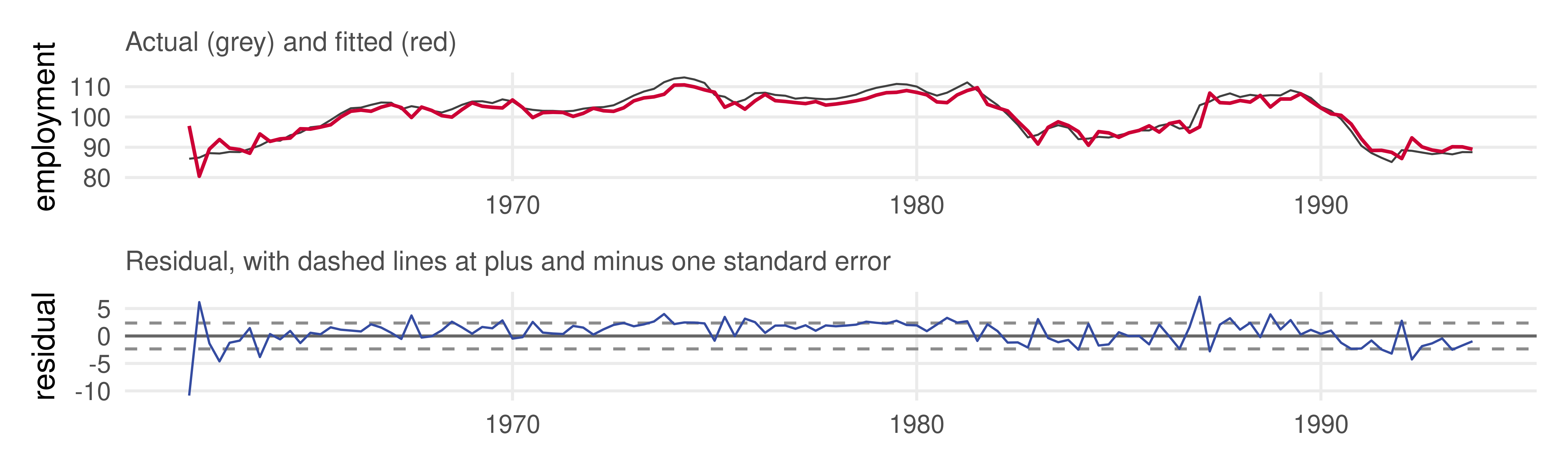
All four coefficients are significant and the fit is invertible. Still, R^2 = 0.90 against 0.96 for the AR(2), the residual standard error is 2.36 against 1.45, and DW = 1.53 signals positive residual autocorrelation.
The book’s Table 7.12a reports a different optimum for the same model (\hat\theta = 1.59, 0.99, -0.02, -0.30, SSR = 1072 against 683 here); exact maximum likelihood gives a third. MA objective functions can have several local optima. Every version tells the same story.
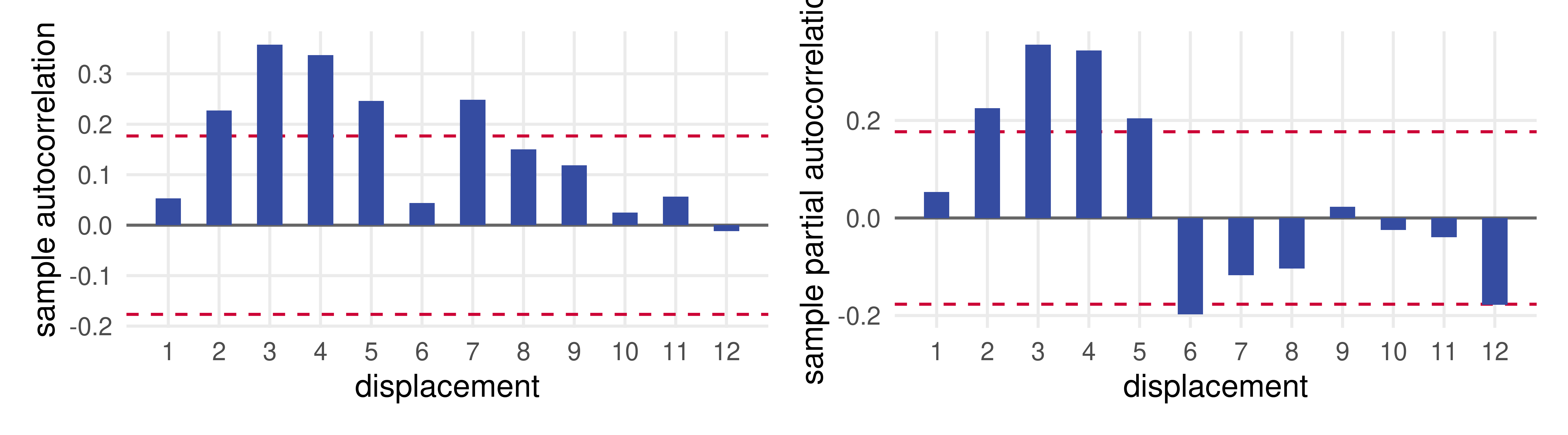
The residual autocorrelations peak at displacements 2 to 5 and the Q statistics reject white noise at every horizon: the MA(4) has missed most of the cycle. Exactly what a four-period memory should be expected to do with a series this persistent.
Diebold’s Figure 7.14. The Q statistics are compared with \chi^2_{m-4}, four MA parameters having been estimated.
The ARMA grid
Fit every ARMA(p,q) with p, q \leq 4 and tabulate AIC and SIC. A fitted MA polynomial can turn out non-invertible; such fits are inadmissible whatever their sum of squares, and the table blanks them.
Twenty-five fits, one call each. admissible checks both root conditions; tab() lays a statistic out with AR order down the rows and MA order across the columns.
SIC selects the AR(2), an ARMA(2,0): the model we already have.
AIC, which penalizes parameters less harshly, selects an ARMA(3,1).
The blanked cells, ARMA(2,3), (3,2), (3,3) and (3,4), had inverse MA roots outside the unit circle. They reach a lower sum of squares only by abandoning invertibility.
Both selections agree with the book’s Tables 7.18a and 7.18b. Let us look at the ARMA(3,1).
Diebold’s Figure 7.18. A CSS fit does not impose invertibility; exact maximum likelihood (next slides) restricts the search to invertible models.
The ARMA(3,1)
a31 <-arima(y, order =c(3, 0, 1), method ="CSS"); a31
##    R2   SER    DW   AIC   SIC
## 0.965 1.432 2.060 0.757 0.868
round(1/polyroot(c(1, -coef(a31)[1:3])), 2); round(-coef(a31)[4], 2) # inverse AR roots; inverse MA root
## [1] 0.93+0i -0.94+0i 0.51+0i
##   ma1
## -0.97
Diebold’s Table 7.19a: the same estimates and the same inverse roots, .93, .51, -.94 and -.97.
A common factor
The ARMA(3,1) looks good: R^2 = 0.965, white-noise residuals, the lowest AIC. Yet apart from that AIC it looks no better than the AR(2), which seemed perfect. Three reasons to prefer the AR(2):
When AIC and SIC disagree, take the more parsimonious model the SIC picks.
A selection strategy that also reads the correlogram points to the AR(2).
The richer dynamics are likely spurious. The ARMA(3,1) has an inverse AR root of -0.94 and an inverse MA root of -0.97. Statistically indistinguishable, they cancel:
an ARMA(2,0) whose roots, 0.93 and 0.51, are those of our AR(2) (0.92 and 0.52).
Look out for common factors: they mean a simpler model, and they make estimation fragile. The exact likelihood of this ARMA(3,1) is nearly flat along the cancelling direction; fable’s maximum-likelihood fit warns about convergence and reports standard errors ten times those above.
The same in fable
ARIMA() fits by maximum likelihood, discards non-stationary and non-invertible candidates, and with stepwise = FALSE searches the full grid.
fit <- samp |>model(ARIMA(Employment ~1+pdq(0:4, 0, 0:4) +PDQ(0, 0, 0), ic ="bic", stepwise =FALSE))report(fit)
The AR(2) again, and also with ic = "aic": under exact likelihood the mixed models lose their edge. fit |> forecast(h = 4) then gives the point forecasts of Lecture 7.
PDQ(0, 0, 0) switches off seasonal terms; 1 asks for a constant. Maximum likelihood estimates the mean at 98.0 rather than 101.2 and the AR coefficients at 1.45 and -0.48.
Point forecasts: MA(4) against AR(2)
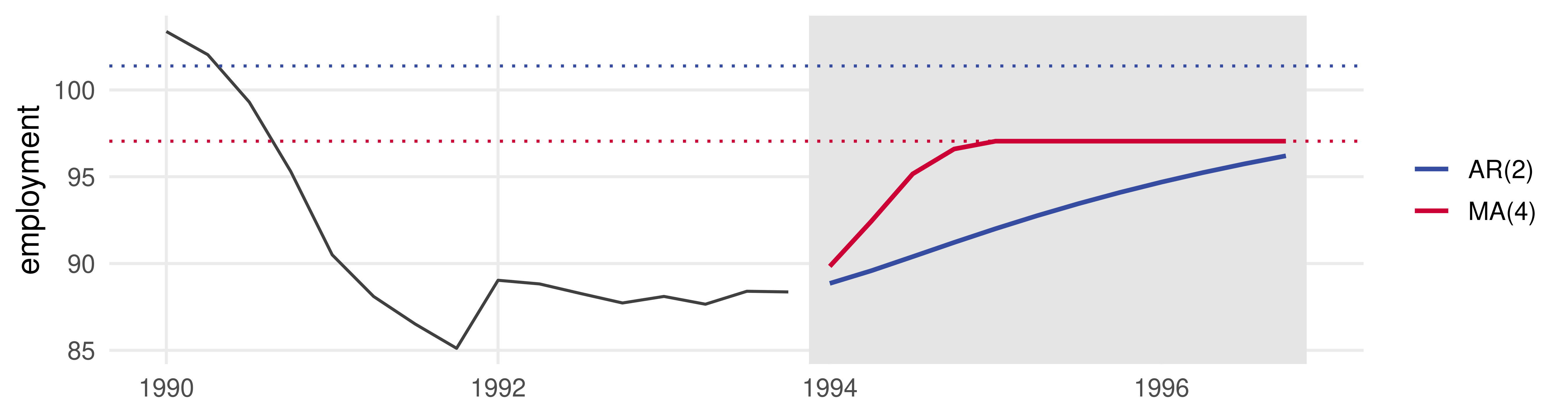
ar2 <-arima(y, order =c(2, 0, 0), method ="CSS")h <-12; qtr <-dec_q(yearquarter("1994 Q1") +0:(h -1))paths <-rbind(data.frame(t = qtr, model ="MA(4)", y =as.numeric(predict(ma4, n.ahead = h)$pred)),data.frame(t = qtr, model ="AR(2)", y =as.numeric(predict(ar2, n.ahead = h)$pred)))means <-data.frame(model =c("MA(4)", "AR(2)"), y =c(coef(ma4)["intercept"], coef(ar2)["intercept"]))
The MA(4) forecast climbs to its mean (dotted) within four quarters and stays there: a four-period memory has nothing to say beyond h = 4. Employment is well below its mean in 1993Q4 and historically very persistent, so a quick rise seems unnatural. The AR(2) reverts slowly, as the data do.
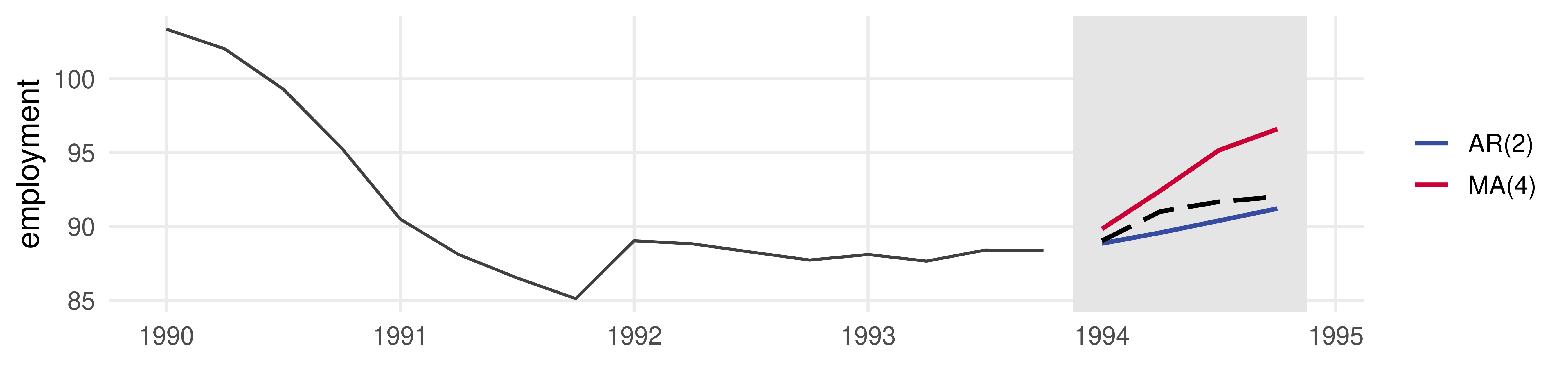
The realization (dashed black) stays well below the mean, as the AR(2) predicted. The MA(4) error is eight times larger, and the ARMA(3,1) gains nothing over the AR(2).
Diebold’s Figures 7.24 and 7.27. The book’s MA(4) optimum does worse still (MSE 55.9); Lecture 7’s OLS AR(2) gave 1.3.
What to take away
Wold’s theorem: every covariance stationary series is an infinite moving average of its innovations. Forecasting models are parsimonious approximations of that representation, rational distributed lags \Theta(L)/\Phi(L).
Signatures. MA(q): ACF cuts off at q, PACF decays, always stationary, invertible under a root condition. AR(p): the mirror image. ARMA: both decay.
Forecasting is one procedure seen from two sides: write the process at T + h, project on \Omega_T. From the MA side, future shocks drop out and the h-step error is an MA(h-1) that cannot be forecast. From the AR side, the chain rule recursion does the same arithmetic, and for ARMA models only the first q steps involve the residuals.
Estimation. MA and ARMA models need numerical least squares or maximum likelihood; autoregressions need OLS, which is consistent but biased by about -(1+3\phi)/T.
Employment. MA(4) misses the cycle; AIC’s ARMA(3,1) hides a common factor; the AR(2) wins on SIC, on the correlogram, and out of sample.
R cheat sheet
library(fpp3)# ---- population properties ----------------------------------------------------ARMAacf(ar =0.7, ma =0.5, lag.max =12) # ACF; pacf = TRUE for the PACFARMAtoMA(ar =0.7, ma =0.5, lag.max =12) # psi weights of the MA(infinity) formMod(1/polyroot(c(1, -phi))) # inverse AR roots; c(1, theta) for MA rootsarima.sim(n =200, list(ar =0.7, ma =0.5)) # simulate# ---- estimation ---------------------------------------------------------------arima(y, order =c(p, 0, q), method ="CSS") # conditional least squares; default "CSS-ML"ic_arma(fit) # R2, SER, DW, AIC, SIC (defined in these slides)correlogram(residuals(fit), m =12, dof = p + q) # residual correlogram (Lecture 7)tsb |>model(ARIMA(y ~1+pdq(p, 0, q) +PDQ(0, 0, 0))) # fable; pdq(0:4, 0, 0:4) + stepwise = FALSE to searchar(y, order.max =1, aic =FALSE, method ="ols") # OLS autoregression; "yw" and "mle" alternatives# ---- point forecasts ----------------------------------------------------------predict(fit, n.ahead = h)$pred # chain rule, done by arima()arma_forecast(const, phi, theta, y, residuals(fit), h) # the same by hand (defined in these slides)model(tsb, ARIMA(y ~1+pdq(2, 0, 0))) |>forecast(h =4) # fable
References
Additional resources
Textbooks
Diebold, F.X. Forecasting in Economics, Business, Finance and Beyond, Chapter 7. The employment application and its data come from the book’s companion files.
Pesaran, M.H. (2015), Time Series and Panel Data Econometrics, Chapter 14, for ARMA algebra and the small-sample bias of OLS (Section 14.5).
Box, G.E.P. and Jenkins, G.M. (1970), Time Series Analysis: Forecasting and Control, Holden-Day. The origin of the identify-estimate-check cycle used in Section 8.
Original sources
Wold, H. (1938), A Study in the Analysis of Stationary Time Series. Kolmogorov, A.N. (1941), “Interpolation and Extrapolation of Stationary Random Sequences,” and Wiener, N. (1949), Extrapolation, Interpolation and Smoothing of Stationary Time Series.
Kendall, M.G. (1954), “Note on Bias in the Estimation of Autocorrelation,” Biometrika, 41, 403–404; Marriott, F.H.C. and Pope, J.A. (1954), “Bias in the Estimation of Autocorrelations,” Biometrika, 41, 390–402.
Quenouille, M.H. (1949), Journal of the Royal Statistical Society B, 11, 68–84; Orcutt, G.H. and Winokur, H.S. (1969), Econometrica, 37, 1–14; Shaman, P. and Stine, R.A. (1988), Journal of the American Statistical Association, 83, 842–848.
Data: data/caemp.csv, seasonally adjusted Canadian employment index, 1961Q1 to 1994Q4, from the companion files.