Lecture 7: Cycles I, Stationarity and Autoregression
Zhan Gao
08 October 2026
The third component
Previously we wrote y_t = T_t + S_t + C_t + \varepsilon_t and dealt with trend and seasonality. Both are deterministic: fixed functions of the calendar, hence trivial to extrapolate.
Every residual plot in that lecture told the same story: what was left over has rich dynamics.
That the third component C_t - the cycle.
Cycles, broadly defined
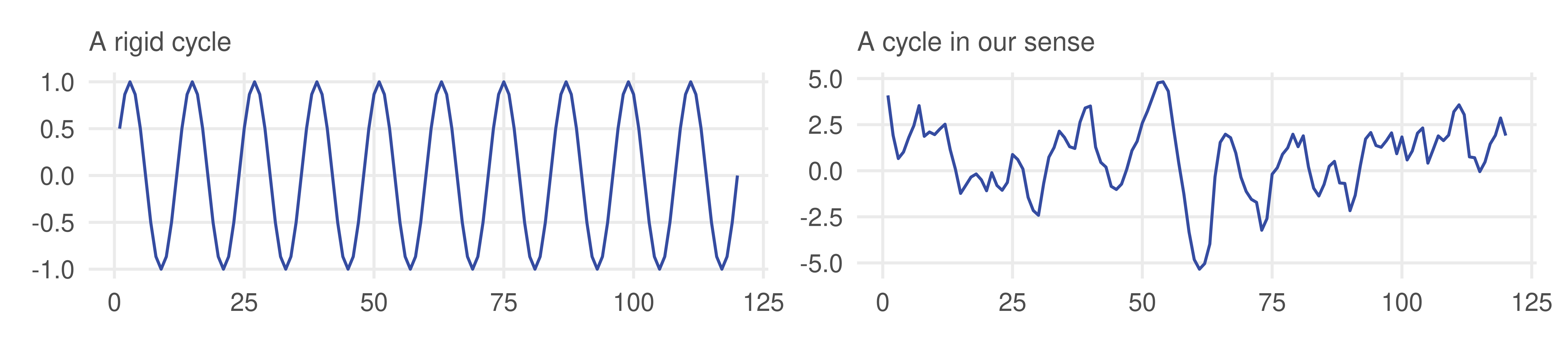
When you hear “cycle” you may picture the rigid up-and-down pattern on the left. Fluctuations in business, finance and economics are rarely that regular.
What we mean by a cycle is any stable, mean-reverting dynamics not captured by the trend or the seasonal: the series is persistent, yet shocks eventually die out and the series returns toward a fixed mean. The right panel qualifies; so does every residual series from the previous lecture.
Today
Trend and seasonal dynamics were simple to model. Cyclical dynamics are richer, and so are the models…
Today:
the language for describing such dynamics (covariance stationarity, autocorrelation)
the simplest model that produces them (the autoregression)
Diebold, Forecasting in Economics, Business, Finance and Beyond, Chapter 6. Sections 1 to 3 also draw on Pesaran (2015), Time Series and Panel Data Econometrics, Chapter 14.
Stationarity
A time series is one realization
A time series is a chronologically ordered collection of random variables. In theory the sequence \ldots, y_{-1}, y_0, y_1, y_2, \ldots runs from the infinite past to the infinite future; what we observe, y_1, \ldots, y_T, is a finite piece of one draw, the sample path.
The observations are dependent: y_t is related to y_{t-1}. Cross-sectional analysis relies on independence across observations. Here the dependence is the object of study, because it is what links the future to the past.
We see a single realization. Statistical analysis needs repeated patterns: something about the process must be the same at t_0 as at t_0 + h.
Strict and weak stationarity
Stationarity requires the “patterns” to be invariant across time.
Strict stationarity. The joint distribution of (y_{t_1}, \ldots, y_{t_k}) equals that of (y_{t_1+h}, \ldots, y_{t_k+h}) for every k, every choice of dates, and every shift h.
Weak, or covariance, stationarity restricts only the first two moments:
E(y_t) = \mu for all t: the mean is constant, so it needs no time subscript;
\gamma(t, \tau) = \operatorname{cov}(y_t, y_{t-\tau}) = \gamma(\tau) for all t: the autocovariance depends only on the displacement \tau, not on the date;
\gamma(0) = \operatorname{var}(y_t) < \infty.
Strict stationarity implies covariance stationarity when the first two moments exist. Everything in this course rests on the weak version.
Because only means and covariances are restricted, covariance stationarity is also called second-order stationarity. It says nothing about skewness, kurtosis, or the shape of the distribution.
The autocovariance function
\gamma(\tau) = E[(y_t - \mu)(y_{t-\tau} - \mu)], viewed as a function of \tau, is the basic summary of a stationary series’ dynamics.
It is symmetric, \gamma(\tau) = \gamma(-\tau): only the displacement matters, not its direction. We plot \tau \geq 0.
\gamma(0) = \operatorname{var}(y_t), and |\gamma(\tau)| \leq \gamma(0) by the Cauchy-Schwarz inequality. A finite variance therefore makes every autocovariance finite.
Its units are the square of the units of y. A covariance of ten million says nothing about the strength of association; a correlation of 0.95 does.
So we standardize. The autocorrelation function is
using that under stationarity both variances equal \gamma(0). Always \rho(\tau) \in [-1, 1] and \rho(0) = 1; only the displacements beyond 0 carry information.
The partial autocorrelation function
The partial autocorrelation at displacement \tau, p(\tau), is the coefficient on y_{t-\tau} in the population linear regression
y_t \;\text{ on }\; y_{t-1},\, y_{t-2},\, \ldots,\, y_{t-\tau} .
Such regressions are called autoregressions: the variable is regressed on its own lags.
The autocorrelation \rho(\tau) is the simple correlation between y_t and y_{t-\tau}.
The partial autocorrelation p(\tau) is the correlation between y_t and y_{t-\tau}after controlling fory_{t-1}, \ldots, y_{t-\tau+1}.
At displacement 1 there is nothing to control for, so p(1) = \rho(1). Beyond it they diverge, and each summarizes the dynamics in its own way.
Like \rho(0), p(0) = 1 by construction. Plots of both functions start at displacement 1.
“Population regression”: imagine an infinite sample, so that the coefficients are the true values, free of sampling variation.
Shapes of autocorrelation functions
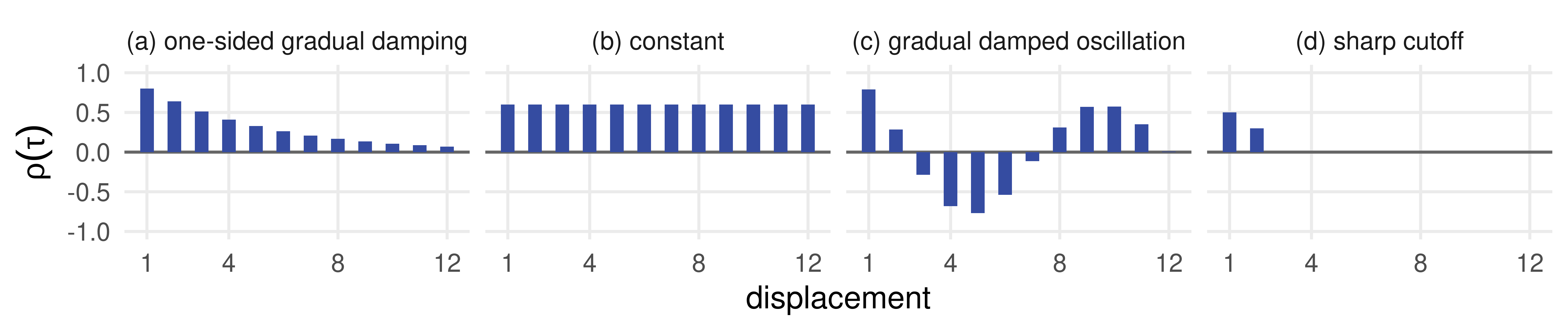
All the processes we study have autocorrelations and partial autocorrelations that approach zero as the displacement grows. How they approach zero is the fingerprint we will read.
Panels (a) and (c): gradual decay, monotone in one case, oscillating in the other.
Panel (d): an abrupt drop to zero beyond some displacement.
Panel (b) is ruled out: a stationary series must eventually forget its past.
Otherwise one realization could never reveal the mean. Strictly this is an ergodicity condition on top of stationarity; Diebold folds it into the definition.
Is nonstationarity fatal?
Many economic series are not covariance stationary. A trend is a mean that rises over time; seasonality is a mean that varies with the season. Both violate requirement 1.
Two strategies make the assumption workable nonetheless:
Model the nonstationary components explicitly, as in later lectures, and treat the cycle that is left over as stationary. That is the plan for most of the course.
Transform. Series nonstationary in levels often look stationary in growth rates.
The tell-tale sign of a trend: a sample ACF that barely decays (left). In growth rates the same data show modest, quickly fading persistence (right).
White noise, and the Wold representation
The fundamental building block
Before estimating anything we need the population properties of a few time series processes. The simplest one is the block from which all others are built:
with the shock \varepsilon_tuncorrelated over time. A process with zero mean, constant variance and no serial correlation is white noise: y_t \sim WN(0, \sigma^2).
Two stronger versions, by adding assumptions:
Independent white noise, y_t \sim \text{iid}(0, \sigma^2): serially independent, not merely uncorrelated. Zero correlation implies independence only in the normal case, so this is a genuine strengthening.
Gaussian white noise, y_t \sim \text{iid}\, N(0, \sigma^2): uncorrelated and normal, hence independent.
The name is by analogy with white light, which contains every color of the spectrum in equal amounts: white noise is composed of cycles of every periodicity, in equal amounts.
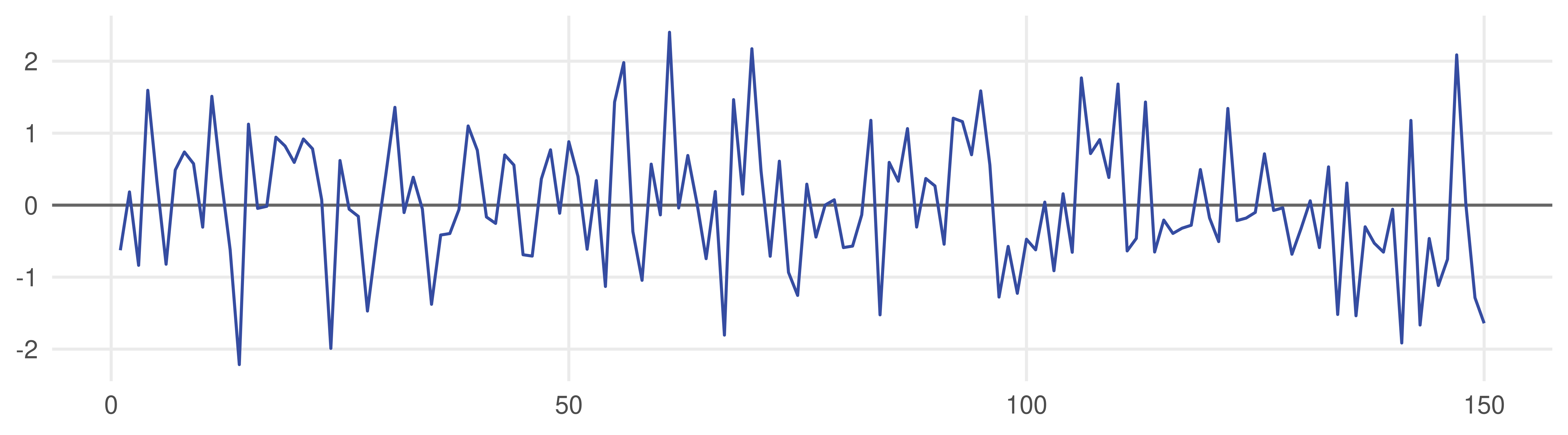
A realization of Gaussian white noise
set.seed(1)wn <-data.frame(t =1:150, y =rnorm(150))ggplot(wn, aes(t, y)) +geom_hline(yintercept =0, colour ="grey40") +geom_line(colour = smu_blue) +labs(x =NULL, y =NULL)
There are no patterns of any kind. Whatever happened last period tells you nothing about this one.
You have met white noise before: the disturbance of a regression model is assumed to be white noise of one sort or another. The difference is that regression disturbances are unobservable, whereas here we are modeling an observed series.
Moments of white noise
Unconditional mean and variance: E(y_t) = 0 and \operatorname{var}(y_t) = \sigma^2, both constant, as they must be for any covariance stationary process.
Because the shocks are uncorrelated, every autocovariance beyond displacement 0 is zero:
The partial autocorrelations vanish for the same reason: a population regression of y_t on y_{t-1}, or on y_{t-1} and y_{t-2}, or on any set of lags, produces nothing but zero coefficients.
Degenerate, yes. Also the reference point: every diagnostic we build asks how far is this series from white noise, and in what direction.
Conditional and unconditional moments
A second way to characterize dynamics: the mean and variance of y_tconditional on its past, \Omega_{t-1} = \{y_{t-1}, y_{t-2}, \ldots\}. For independent white noise,
Conditional and unconditional moments coincide: there are no dynamics.
For a process with dynamics they differ. Unconditional moments must be constant, by stationarity. Conditional moments move with the information set: expected laptop sales growth next quarter may be ten percent unconditionally, but much higher given that sales grew twenty percent this quarter.
The conditional mean is exactly the object Lecture 4 called the optimal forecast under quadratic loss. Time series modeling is the business of computing it.
Why white noise matters
It is the building block. Processes with much richer dynamics are simple transformations of white noise. The next slide makes that precise.
It is the target. The goal of time series modeling, and of one-step-ahead forecasting, is to reduce the data to white noise. If the one-step forecast errors are not white noise, they are serially correlated, hence forecastable, hence the forecast can be improved.
A good model leaves behind residuals you cannot forecast.
So we need to recognize white noise when we see it, and to test for it.
The Wold representation (a preview)
Wold (1938). Let y_t be covariance stationary with any deterministic part d_t (a constant, a trend, seasonals) removed. Then
where \varepsilon_t is the innovation, the part of y_t that the linear past cannot predict, and \varepsilon_t \sim WN(0, \sigma^2).
Read it as: every stationary process is white noise passed through a linear filter. Infinitely many coefficients look hopeless for estimation with finite data. They are not, because parsimonious models (autoregressions, coming up) imply particular sequences b_j with only a few free parameters.
Summable coefficients keep the process stable
Suppose the coefficients decay fast enough to be absolutely summable, \sum_j |b_j| < \infty (exponential decay is the leading case). Then, with d_t = 0:
The autocovariances are \gamma(\tau) = \operatorname{cov}\Big(\sum_j b_j \varepsilon_{t-j}, \sum_k b_k \varepsilon_{t-\tau-k}\Big) = \sigma^2 \sum_{j=0}^{\infty} b_j\, b_{j+\tau}, because E(\varepsilon_{t-j}\varepsilon_{t-\tau-k}) = \sigma^2 only when j = k + \tau and is 0 otherwise.
They are absolutely summable too: \sum_{\tau=0}^{\infty} |\gamma(\tau)| \leq \sigma^2 \sum_{\tau} \sum_{j} |b_j|\,|b_{j+\tau}| \leq \sigma^2 \Big(\sum_j |b_j|\Big)^2 < \infty, so \rho(\tau) \to 0: the process forgets. This is the decay we asked for.
The long-run variance, \lim_{T\to\infty} \operatorname{var}\big(\sqrt{T}\,\bar y\big) = \sum_{\tau=-\infty}^{\infty} \gamma(\tau), is finite. It is what replaces \sigma^2 in the standard error of a time series mean.
The sample correlogram and Q tests
The analog principle
Now we have data, and here is how to do model-free chracterizatino of the dynamics of the observed time series. The analog principle: estimate population moments by replacing expectations with sample averages.
The sum starts at t = \tau + 1 because y_{t-\tau} must exist, yet we divide by T, not T - \tau. When T is large relative to \tau it hardly matters, and dividing by T has a technical advantage.
\hat\rho(\tau) as a function of \tau is the sample autocorrelation function, or correlogram.
The sample partial autocorrelation replaces the population regression by the feasible one: fit \hat y_t = \hat c + \hat\beta_1 y_{t-1} + \cdots + \hat\beta_\tau y_{t-\tau} by OLS and set \hat p(\tau) = \hat\beta_\tau. Again \hat p(1) = \hat\rho(1).
Dividing by T makes the sequence \hat\gamma(0), \hat\gamma(1), \ldots positive semidefinite, like every true autocovariance function. Dividing by T - \tau does not guarantee that.
Sampling distribution under white noise
A key result, which we simply assert: if y is white noise, then in large samples
and the sample autocorrelations at different displacements are approximately independent.
Mean zero: \hat\rho(\tau) is unbiased for the true value, which is zero.
Standard deviation 1/\sqrt{T}: easy to construct and to remember.
So about 95% of the sample autocorrelations of a white noise series fall within 0 \pm 2/\sqrt{T}. These are the two-standard-error bands drawn on every correlogram. The same result and the same bands hold for \hat p(\tau).
The bands judge one displacement at a time. Usually the question is joint: is the whole autocorrelation function zero?
From bands to a joint test
Rewrite the result as \sqrt{T}\,\hat\rho(\tau) \sim N(0,1) and square it: T\hat\rho^2(\tau) \sim \chi^2_1. Squaring stops positive and negative values from cancelling when we add them up.
Sum m approximately independent \chi^2_1 variables and you get a \chi^2_m. Hence the Box-Pierce Q statistic
Q_{BP} = T \sum_{\tau=1}^{m} \hat\rho^2(\tau) \;\overset{d}{\sim}\; \chi^2_m,
\quad \text{ under } H_0: \rho(1) = \cdots = \rho(m) = 0
in large samples.
Its finite-sample behavior is poor. A reweighting that follows the \chi^2_m more closely in small samples is the Ljung-Box Q statistic
The weights (T+2)/(T-\tau) are near 1 for large T, so the two rarely disagree.
Choosing m. Too small and the test ignores most of the autocorrelation function; too large relative to T and the \chi^2 approximation deteriorates. m near \sqrt{T} is a reasonable rule of thumb.
The correlogram in a few lines of R
Base R already computes each piece: acf(), pacf(), and Box.test(). Assembling them into the table a textbook prints takes one small function, which we will reuse all day.
correlogram <-function(x, m =12, dof =0) { T <-length(x) a <-acf(x, lag.max = m, plot =FALSE)$acf[-1] # rho_hat(1), ..., rho_hat(m) p <-pacf(x, lag.max = m, plot =FALSE)$acf[, 1, 1] # p_hat(1), ..., p_hat(m) Q <- T * (T +2) *cumsum(a^2/ (T -1:m)) # Ljung-Box, for m = 1, 2, ... pv <-pchisq(Q, df =pmax(1:m - dof, 1), lower.tail =FALSE) pv[1:m <= dof] <-NA# no p-value until m > dofdata.frame(lag =1:m, acf =round(a, 3), pacf =round(p, 3), Q =round(Q, 2), p =round(pv, 4))}
dof is for later: when x is a residual from a model with dof estimated parameters, the null distribution of Q is better approximated by \chi^2_{m - \text{dof}}.
acf() divides by T, exactly as on the previous slide. corr_plot(), the bar-chart helper used below, is defined in the source of these slides.
A process whose truth we know
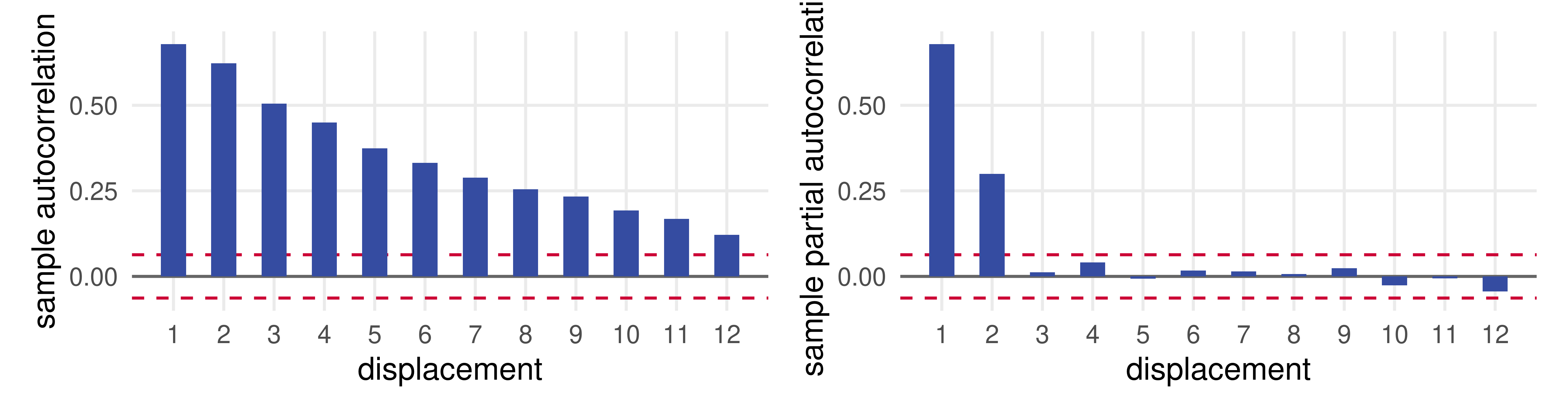
Simulate a series with dynamics, an autoregression of order two (the model is explained later), and look at its correlogram.
The dashed lines are \pm 2/\sqrt{1000} = \pm 0.063. The sample autocorrelations decay gradually and stay far outside the bands for many displacements; the partial autocorrelations are large at 1 and 2 and negligible beyond. Remember that shape.
Q tests on the simulated series
Box.test(y, lag =10, type ="Box-Pierce")
##
##  Box-Pierce test
##
## data:  y
## X-squared = 1795.5, df = 10, p-value < 2.2e-16
Box.test(y, lag =10, type ="Ljung-Box")
##
##  Box-Ljung test
##
## data:  y
## X-squared = 1805.3, df = 10, p-value < 2.2e-16
Both reject white noise beyond any doubt, and they barely differ: T = 1000 is large. For contrast, a fresh draw of pure noise:
set.seed(321); Box.test(rnorm(1000), lag =10, type ="Ljung-Box")$p.value
## [1] 0.173089
Application: Canadian employment I
The Canadian employment data
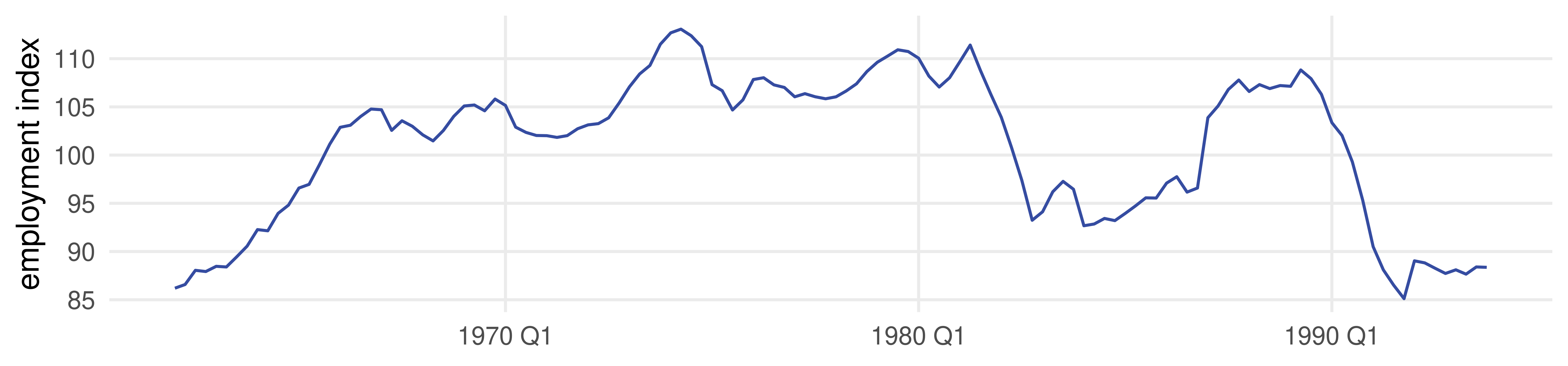
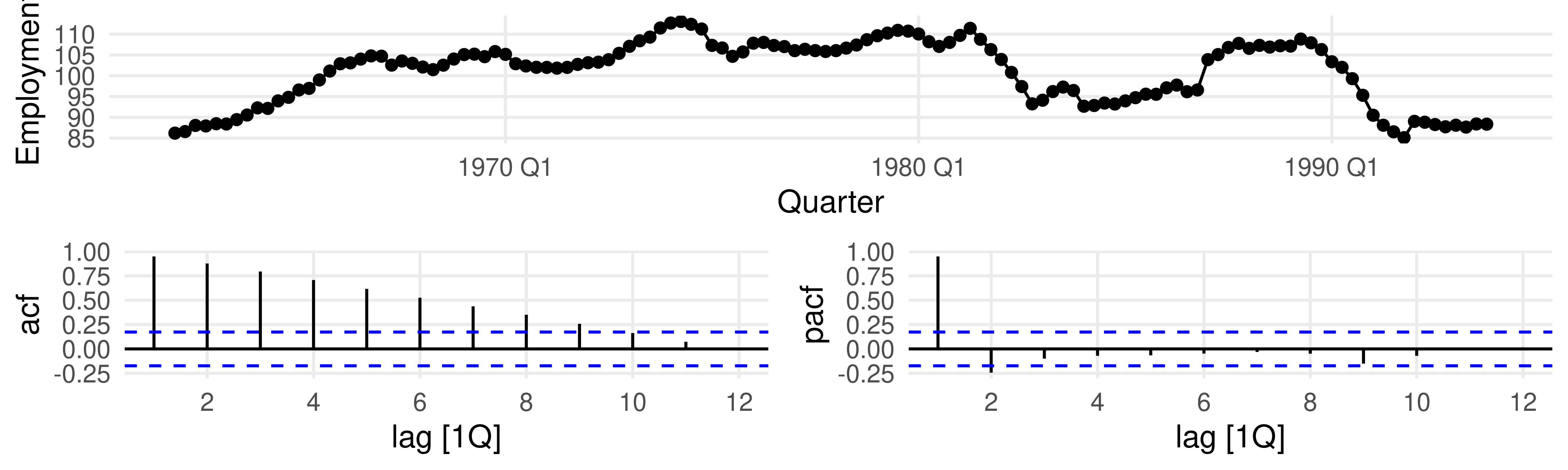
A quarterly, seasonally adjusted index of Canadian employment, 1962Q1 to 1993Q4 (T = 128). The file also holds 1961 and 1994, which we keep aside: 1961 supplies pre-sample lags, 1994 is the realization we will forecast.
No trend, and no seasonality because the series is seasonally adjusted. But it is highly serially correlated: it evolves slowly, high in booms and low in the recessions of the early 1980s and early 1990s.
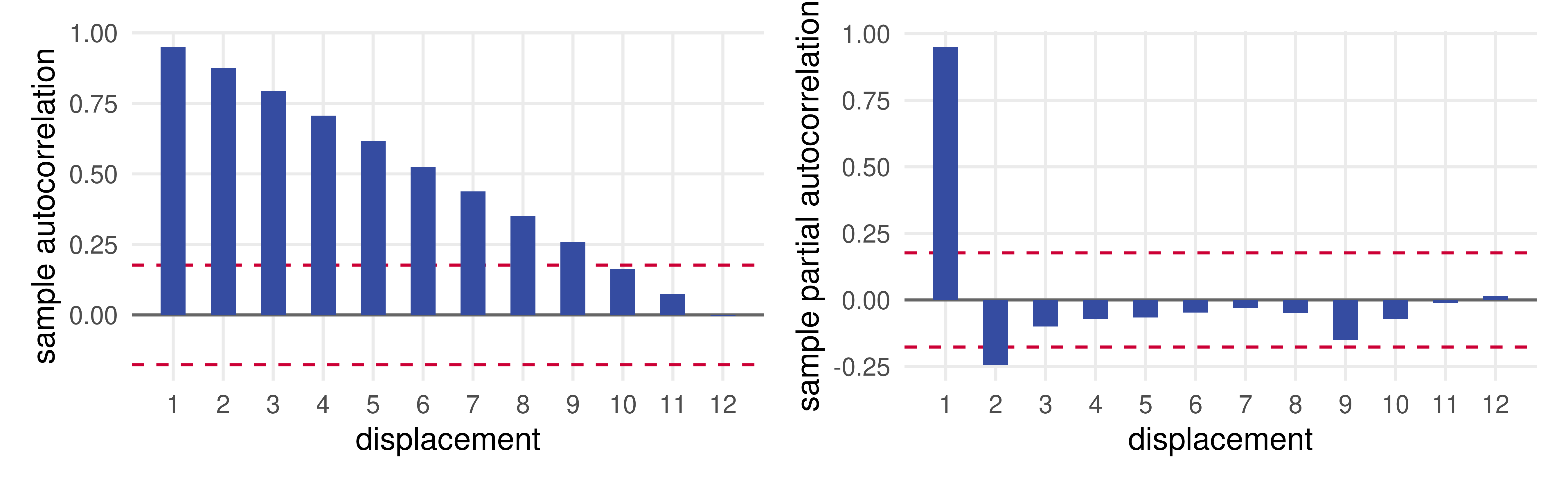
The two-standard-error band is 2/\sqrt{128} = 0.18. Each row’s Q uses the autocorrelations up to that displacement.
Reading the table
Q statistics. For every m from 1 to 12 the p-value is zero to four decimals: the white noise hypothesis is decisively rejected. Employment has a cyclical component.
Sample autocorrelations. Very large relative to the 0.18 standard error, and they display slow, one-sided decay: 0.95, 0.88, 0.80, 0.71, \ldots
Sample partial autocorrelations. Large at displacement 1 (equal to the autocorrelation, necessarily) and clearly negative at displacement 2 (-0.24), then statistically negligible.
Gradual autocorrelation decay together with a partial autocorrelation function that cuts off at displacement 2 is a particular shape. Such shapes suggest candidate models, and
Many time series models can be easily written in the language of the lag operatorL, which lags a series: L y_t = y_{t-1}, L^2 y_t = L(L y_t) = y_{t-2}, and L^m y_t = y_{t-m}.
Usually we operate with a polynomial in L,
B(L) = b_0 + b_1 L + b_2 L^2 + \cdots + b_m L^m ,
so that B(L) y_t = b_0 y_t + b_1 y_{t-1} + \cdots + b_m y_{t-m}, a weighted sum of current and past values called a distributed lag.
The first-difference operator is a first-order lag polynomial: \Delta y_t = (1 - L) y_t = y_t - y_{t-1}.
Infinite order is allowed: B(L)\varepsilon_t = \sum_{i=0}^{\infty} b_i \varepsilon_{t-i}. The Wold representation is exactly B(L)\varepsilon_t with b_0 = 1.
Most time series models contain distributed lags, because they say how the past evolves into the present. The notation is shorthand for stating and manipulating them.
Where you have already met the AR(1)
The Durbin-Watson setting was a regression with serially correlated disturbances. Strip it to an intercept only:
A regression with serially correlated disturbances and no lagged dependent variable is mathematically identical to one with a lagged dependent variable and iid disturbances. Each device mops up the serial correlation the other regressors leave behind; here there are no other regressors at all.
A stochastic difference equation: the current value is a linear function of the previous value plus a shock.
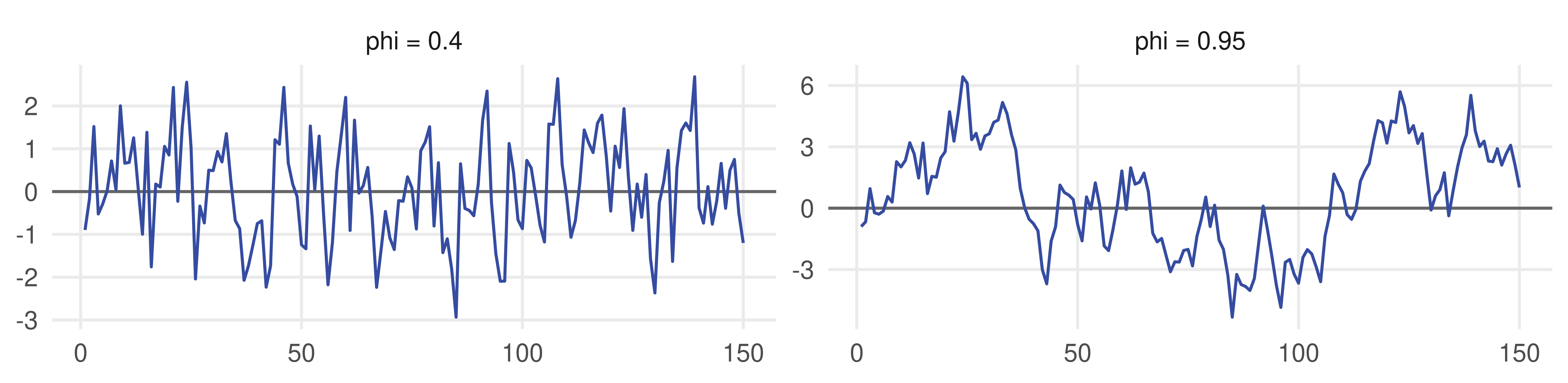
set.seed(2); e <-rnorm(150) # one shock sequence for bothar1 <-function(phi) as.numeric(stats::filter(e, phi, method ="recursive"))d <-data.frame(t =rep(1:150, 2), phi =rep(c("phi = 0.4", "phi = 0.95"), each =150),y =c(ar1(0.4), ar1(0.95)))ggplot(d, aes(t, y)) +geom_hline(yintercept =0, colour ="grey40") +geom_line(colour = smu_blue) +facet_wrap(~ phi, scales ="free_y") +labs(x =NULL, y =NULL)
Same shocks, different \phi. With \phi = 0.95 the fluctuations are far more persistent: the AR(1) can capture highly persistent dynamics with a single parameter.
When is the AR(1) covariance stationary?
The condition, for any autoregression: all roots of the autoregressive lag polynomial lie outside the unit circle. For the AR(1) the polynomial is 1 - \phi L, its root is L = 1/\phi, and |1/\phi| > 1 if and only if |\phi| < 1.
This is the Wold representation with b_i = \phi^i, absolutely summable. Ultimately the shocks are the only things that move y, so y can be written as a weighted history of shocks, with geometrically fading weights. If |\phi| \geq 1 the weights do not fade and no such representation exists.
Unconditional and conditional moments
From the moving-average representation, with \varepsilon uncorrelated across dates,
The conditional mean adapts to the information set as the process evolves. That is the forecast.
The conditional variance \sigma^2 is smaller than the unconditional \sigma^2/(1-\phi^2): knowing the past reduces uncertainty, by a factor that grows with |\phi|.
With an intercept, y_t = c + \phi\, y_{t-1} + \varepsilon_t, the mean is \mu = c/(1-\phi) and everything else goes through for y_t - \mu.
Autocovariances: the Yule-Walker equation
Multiply the process by y_{t-\tau} and take expectations:
because \varepsilon_t is uncorrelated with everything before t, so E(\varepsilon_t y_{t-\tau}) = 0 for \tau \geq 1.
A recursion: given \gamma(\tau) it delivers \gamma(\tau + 1). The initial condition is the variance we just computed, \gamma(0) = \sigma^2/(1-\phi^2), so
Gradual decay, one-sided if \phi > 0 and oscillating if \phi < 0. Positive \phi is the relevant case in economics.
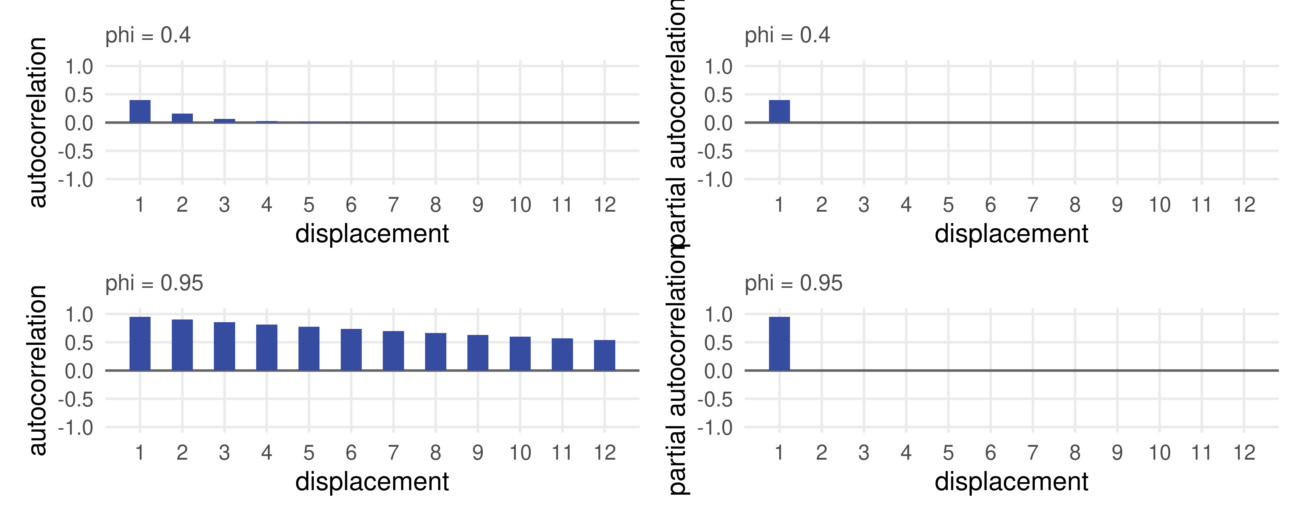
Sharp cutoff in the PACF: p(1) = \phi and p(\tau) = 0 for \tau > 1. The partial autocorrelations are the last coefficients of ever longer population autoregressions; if the truth is an AR(1), the first is \phi and every later one is zero.
Population ACF and PACF of two AR(1) processes
Diebold’s Figures 6.12 to 6.15. Persistence is far stronger at \phi = 0.95; both PACFs cut off after displacement 1.
or \Phi(L)\, y_t = (1 - \phi_1 L - \phi_2 L^2 - \cdots - \phi_p L^p)\, y_t = \varepsilon_t.
Its properties parallel the AR(1) case, and we state them without derivation:
Stationarity: covariance stationary if and only if all roots of \Phi(L) lie outside the unit circle. A quick necessary check is \sum_i \phi_i < 1: if it fails, the process cannot be stationary.
Autocorrelations decay gradually, as for the AR(1), but the patterns are richer.
Partial autocorrelations cut off sharply at displacement p, for the same reason as before.
The Canadian employment correlogram, gradual decay with a PACF cutoff at 2, is therefore the fingerprint of an AR(2).
Yule-Walker for the AR(2)
Multiply y_t = \phi_1 y_{t-1} + \phi_2 y_{t-2} + \varepsilon_t by y_{t-\tau} and take expectations:
Replacing \gamma by \hat\gamma gives the Yule-Walker estimator. We will use OLS instead, but the idea that autocovariances identify the parameters is worth keeping.
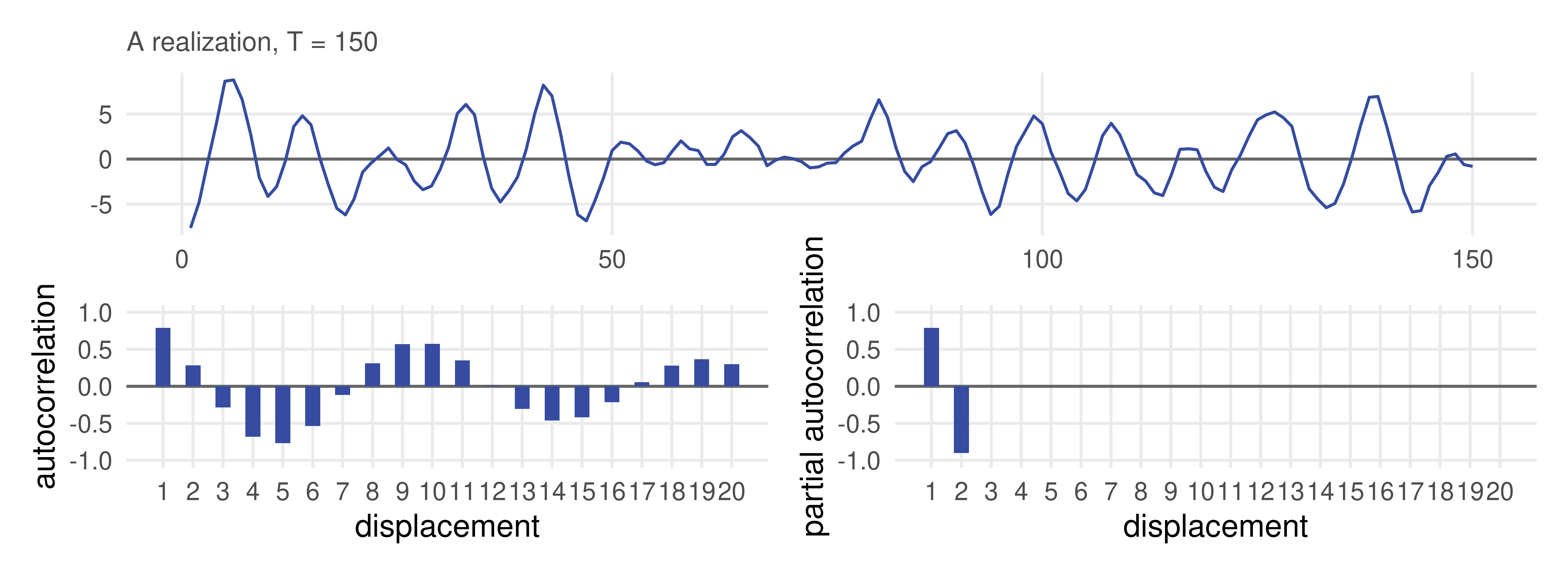
Complex roots: genuine cycles
In the AR(1), oscillation needs \phi < 0 and flips sign every period. Higher-order autoregressions can oscillate with longer, smoother periods, reminiscent of cycles in the traditional sense. That happens when some roots of \Phi(L) are complex. Take
r <-polyroot(c(1, -1.5, 0.9)); r # the two roots, a conjugate pair
## [1] 0.8333333+0.6454972i 0.8333333-0.6454972i
Mod(1/ r) # inverse roots: inside the unit circle
## [1] 0.9486833 0.9486833
2* pi /acos(1.5/ (2*sqrt(0.9))) # period of the implied cycle
## [1] 9.533584
The inverse roots 0.75 \pm 0.58i have modulus 0.95: stationary, but close to the boundary, so the oscillation damps slowly, with a period of about nine and a half quarters.
An AR(2) with complex roots, seen
Diebold’s Figure 6.16. The autocorrelation function oscillates with the period computed on the previous slide, and the PACF still cuts off at 2.
Estimating autoregressions
The sum of squares of an AR(p) is linear in the parameters, so estimation is an ordinary least squares regression of y_t on y_{t-1}, \ldots, y_{t-p} (and a constant). Nothing new to learn.
With lagged dependent variables OLS is consistent, though not unbiased, under stationarity; the usual t and F statistics are valid in large samples.
Order selection. The correlogram suggests candidates. AIC and SIC, choose among them, provided every candidate is fit to the same observations. We keep the pre-sample values as lags so that all orders use all T observations.
fit_stats <-function(m) { e <-residuals(m); y <-fitted(m) +residuals(m) T <-length(e); k <-length(coef(m)); ssr <-sum(e^2)c(R2 =1- ssr /sum((y -mean(y))^2), SER =sqrt(ssr / (T - k)),DW =sum(diff(e)^2) / ssr,AIC =log(ssr / T) +2* k / T, SIC =log(ssr / T) + k *log(T) / T)}
Application: Canadian employment II
AR(1) to AR(4) by OLS
Build the lags on the full file, then restrict to 1962Q1 to 1993Q4. The lags of the first observations are the 1961 values, so every model below has T = 128.
Both AIC and SIC pick the AR(2), in agreement with the correlogram. The third and fourth lags lower the sum of squares by almost nothing and pay a penalty for it.
##           mean inverse_roots1 inverse_roots2
##    101.2412730      0.9221189      0.5166914
Both lags are highly significant: \hat\phi_1 = 1.44, \hat\phi_2 = -0.48. The implied mean \hat c/(1 - \hat\phi_1 - \hat\phi_2) = 101.24 is close to the sample mean of 101.02.
The inverse roots are real, 0.92 and 0.52, inside the unit circle: stationary, no oscillation, and the root at 0.92 is the source of the persistence.
R^2 = 0.96, SER = 1.45, DW = 2.07.
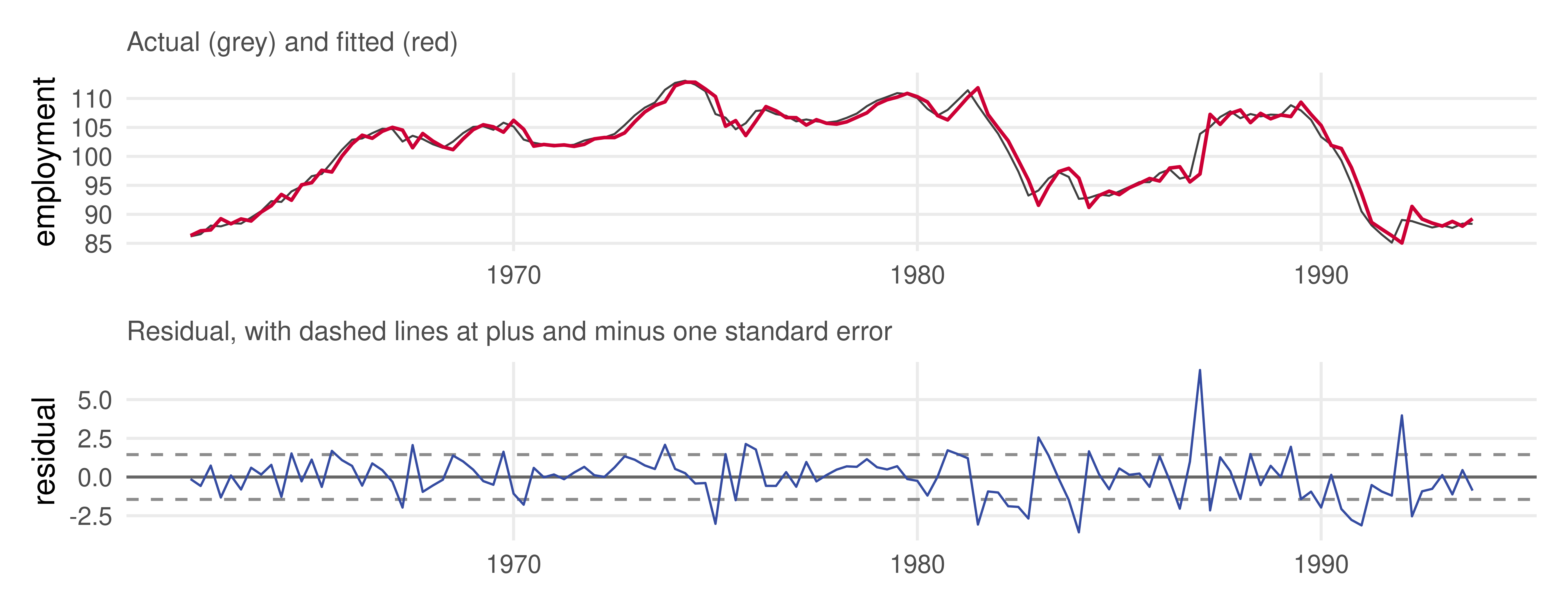
Actual, fitted and residuals
Diebold’s Figure 6.17b. The residuals look like white noise: no runs, no drift, one large positive shock in 1987.
Residual correlogram
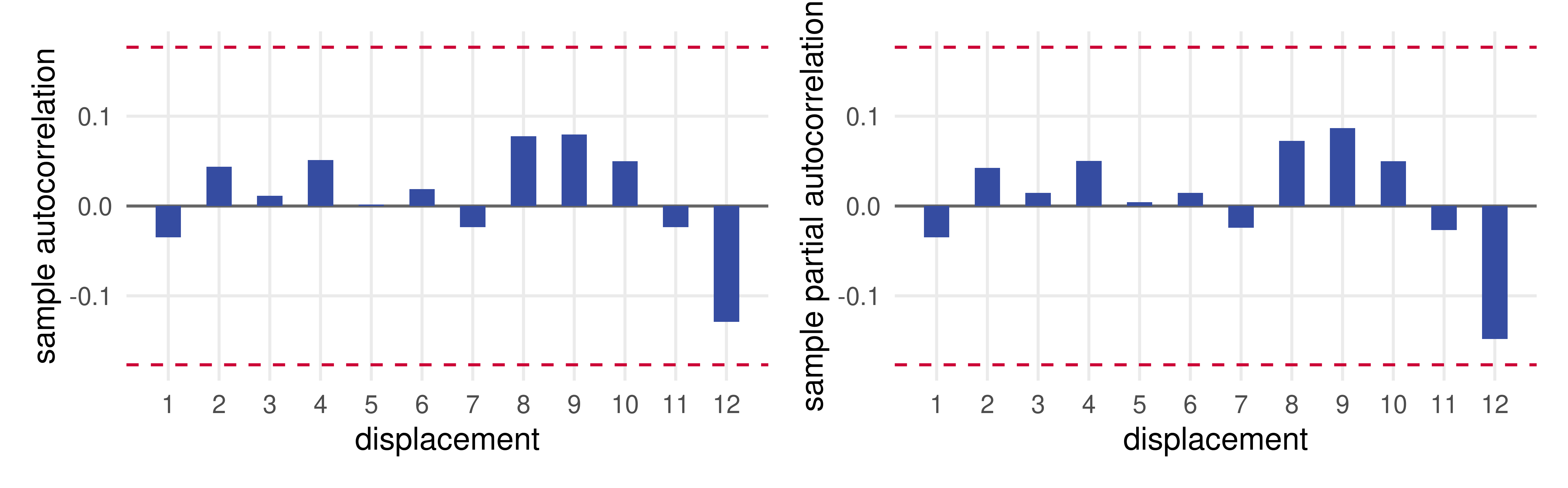
Is what is left over white noise? Two parameters were estimated, so the Q statistics are compared with \chi^2_{m-2} and there is no p-value until m > 2.
Every autocorrelation is inside \pm 0.18 and every p-value is large. The AR(2) has extracted all the linear dynamics.
Residual correlogram, plotted
corr_plot(residuals(ar2), lag_max =12)
The same in fable
AR() in fable fits the same OLS regression. It drops the first p observations of whatever data it is given, so hand it the two 1961Q3 to 1961Q4 quarters as well to reproduce the estimates above exactly.
## # A mable: 1 x 1
##   `AR(Employment ~ order(1:4), ic = "bic")`
##                                     <model>
## 1                           <AR(2) w/ mean>
Forecasting with autoregressions: Wold’s chain rule
The FRV problem, revisited
Recall four ways out of the forecasting-the-right-hand-side-variables problem. Deterministic regressors were the fourth. The third was lagged regressors:
is immediately usable one step ahead, because the regressor for y_{T+1} is x_T, already observed. More lags are fine; the key is that everything on the right is lagged at least one period.
For h steps ahead, model (2) seems to bring the problem back: we would need x_{T+h-1}, so everything on the right would have to be lagged by h periods, not one.
For autoregressions the problem dissolves. A model with y_t on y_{t-1} can be turned into a model with y_t on y_{t-h}, mechanically, for any h. That is Wold’s chain rule.
Information sets, conditional expectations, linear projections
The time-T information set is the observed history, \Omega_T = \{y_T, y_{T-1}, y_{T-2}, \ldots\}, imagined for theory as extending into the infinite past.
Under quadratic loss the optimal forecast of y_{T+h} is the conditional mean E(y_{T+h} \mid \Omega_T). In general it need not be a linear function of the elements of \Omega_T.
Linear functions are tractable, so we work with the best linear approximation to the conditional mean, the linear projectionP(y_{T+h} \mid \Omega_T): the “linear least squares forecast”. Often it is very close to the conditional mean, and in the Gaussian case the two coincide exactly:
The forecast reverts geometrically to the unconditional mean. With an intercept, y_{T+h,T} = c + \phi\, y_{T+h-1,T} \to \mu = c/(1-\phi).
The chain rule for the AR(p)
The same recursion works for any order: write the process at T+h, replace future shocks by 0 and future y’s by their already-computed forecasts,
y_{T+h,T} = c + \phi_1\, y_{T+h-1,T} + \cdots + \phi_p\, y_{T+h-p,T}, \qquad y_{s,T} = y_s \text{ for } s \leq T .
Only the p most recent observations are ever needed, at any horizon. The FRV problem is solved for autoregressions, as it was for cross sections, trends and seasonals.
In truth the parameters are unknown, so we insert the OLS estimates to obtain operational forecasts. The recursion is six lines of R:
# coef = c(c, phi_1, ..., phi_p); y_last = the last p observations, oldest firstchain_rule <-function(coef, y_last, h) { p <-length(coef) -1; path <- y_last; f <-numeric(h)for (i in1:h) { f[i] <- coef[1] +sum(coef[-1] *rev(tail(path, p))) # phi_1 * most recent, phi_2 * the one before, ... path <-c(path, f[i]) # the forecast joins the history } f}
Forecast errors and their variances
The chain rule delivers point forecasts. For interval and density forecasts we need the h-step forecast error variance \sigma_h^2 = \operatorname{var}(y_{T+h} \mid \Omega_T). For the AR(1):
Errors. Subtract the forecast from the outcome and use the moving-average representation:
The limit is the unconditional variance of the process: conditioning information loses its value as the horizon grows, until the forecast is no better than the unconditional mean.
Under normality, y_{T+h} \mid \Omega_T \sim N(y_{T+h,T}, \sigma_h^2) is the density forecast, and y_{T+h,T} \pm 1.96\, \sigma_h the 95% interval.
Higher orders: the moving-average weights
For an AR(p) the error is again a weighted sum of the future shocks, e_{T+h,T} = \sum_{i=0}^{h-1} \psi_i\, \varepsilon_{T+h-i}, where the \psi_i are the coefficients of the process’s moving-average representation y_t = \mu + \sum_i \psi_i \varepsilon_{t-i}. They follow from the AR coefficients by the recursion
psi_weights <-function(phi, h) { psi <-c(1, numeric(h -1)); p <-length(phi)if (h >1) for (j in2:h) for (i in1:min(j -1, p)) psi[j] <- psi[j] + phi[i] * psi[j - i] psi}
Two things the formula ignores. Parameter estimation error, which can make \sigma_h^2 grow without bound rather than converge. And non-normality, which simulation handles without any variance calculation.
Application: Canadian employment III
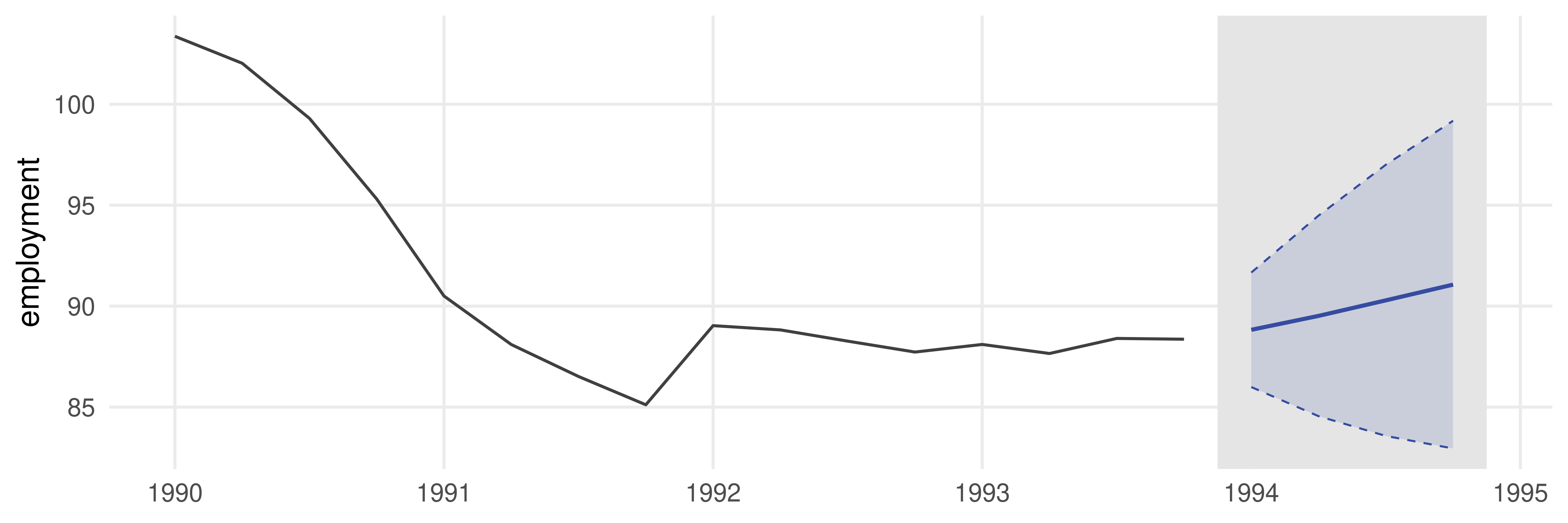
Four quarters ahead
The best autoregression was the AR(2). Its last two observations are 1993Q3 and 1993Q4; feed them to the chain rule and scale the \psi weights by the SER.
b <-coef(ar2); s <-sigma(ar2)fc4 <-chain_rule(b, tail(est$Employment, 2), h =4)se4 <- s *sqrt(cumsum(psi_weights(b[-1], 4)^2))f4 <-data.frame(Quarter =yearquarter("1994 Q1") +0:3, point = fc4, se = se4,lower = fc4 -1.96* se4, upper = fc4 +1.96* se4)round(f4[, -1], 2)
The point forecast climbs slowly from the last observation (88.4) toward the mean (101.2) and is still far below it after four quarters. The standard error grows from the SER to nearly three times the SER, and the bands are nowhere near their long-run width. Both reflect the persistence the AR(2) captured.
History and forecast
Diebold’s Figure 6.20. History 1990Q1 to 1993Q4, then the four-quarter forecast (blue) with its 95% interval.
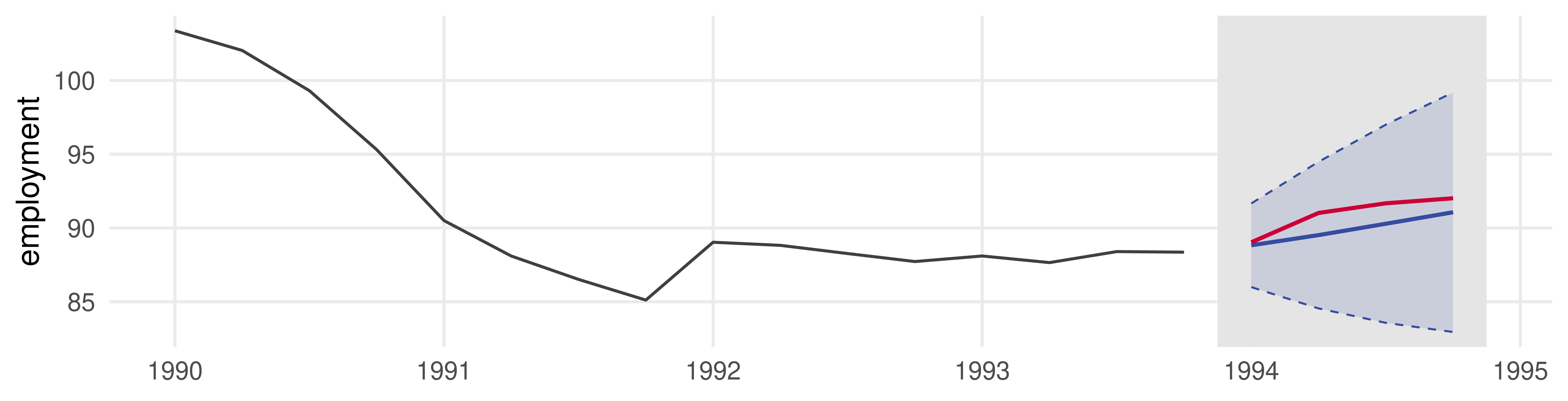
Forecast and realization
real <- emp |>filter(year(Quarter) ==1994) |>as_tibble() |>transmute(t =dec_q(Quarter), y = Employment)fc_plot(recent, f4, actual = real, ylab ="employment")
mean((real$y - f4$point)^2) # mean squared forecast error
## [1] 1.279815
The forecast tracks the recovery well: the realization (red) sits close to the point forecast and well inside the band, with a mean squared error of 1.3, less than the SER squared.
Diebold’s Figure 6.21.
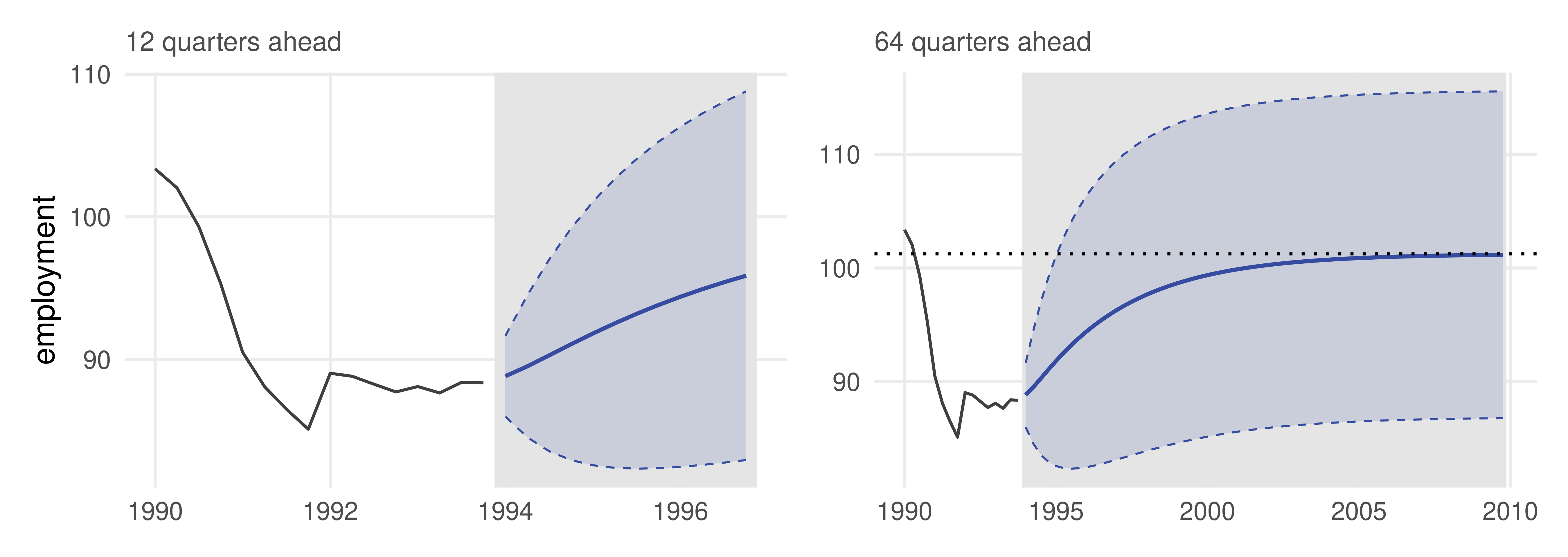
Longer horizons
Eventually the forecast reaches the unconditional mean (dotted) and the bands go flat at \pm 1.96 \times 7.3, the standard deviation the model implies (the sample standard deviation is 7.5). But only after many years: high persistence means a long memory.
Diebold’s Figures 6.22 and 6.23.
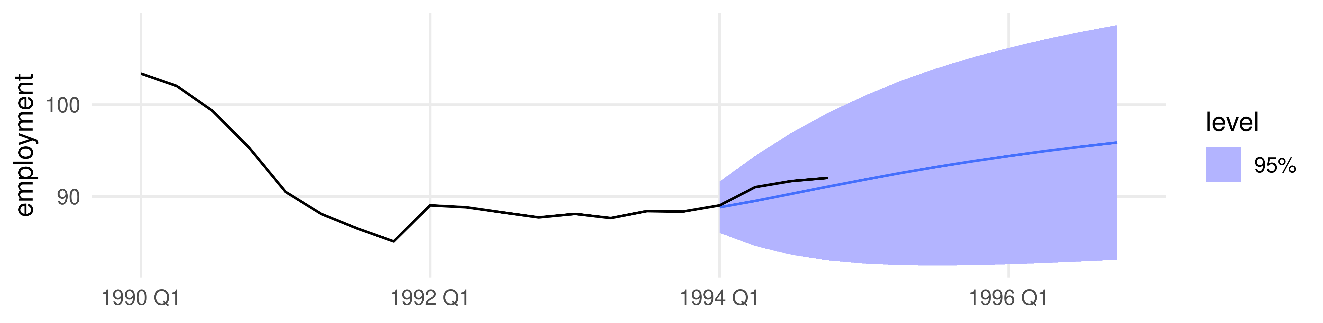
The same in fable
fit |>forecast(h =4) |>hilo(95) |>select(Quarter, .mean, `95%`)
fit |>forecast(h =12) |>autoplot(emp |>filter(year(Quarter) >=1990), level =95) +labs(x =NULL, y ="employment")
fable estimates \sigma^2 by SSR/T rather than SSR/(T-k), so its intervals are about one percent narrower.
What to take away
Covariance stationarity (constant mean, autocovariances that depend only on the displacement, finite variance) is what makes one realization informative about the process. Model the trend and seasonal first, or transform; then treat the cycle as stationary.
White noise has no dynamics. It is the building block of every process (Wold) and the target for every model’s residuals.
The correlogram (sample ACF, PACF, Q statistics with \pm 2/\sqrt{T} bands) is model-free evidence about dynamics. Gradual ACF decay with a PACF cutoff at p points to an AR(p); AIC and SIC settle the order.
An AR(p) is OLS on p lags. It is stationary when the roots of \Phi(L) lie outside the unit circle; for the AR(1), \rho(\tau) = \phi^\tau.
Wold’s chain rule produces forecasts at any horizon by recursion. They revert to the mean, and the forecast-error variance rises from \sigma^2 to the unconditional variance.
R cheat sheet
library(fpp3)# ---- correlogram ----------------------------------------------------------------acf(y, lag.max =12); pacf(y, lag.max =12) # base R (divide-by-T estimator)Box.test(y, lag =12, type ="Ljung-Box") # Q test; fitdf = k for residualscorrelogram(y, m =12, dof =0) # table of acf, pacf, Q, p (defined in these slides)tsb |>gg_tsdisplay(y, plot_type ="partial") # series + ACF + PACF, fpp3tsb |>features(y, ljung_box, lag =12, dof =0) # Ljung-Box, fpp3# ---- autoregressions ------------------------------------------------------------tsb <- tsb |>mutate(L1 =lag(y), L2 =lag(y, 2)) # build lags, then filter to the samplelm(y ~ L1 + L2, data = tsb); fit_stats(fit) # OLS; R2, SER, DW, AIC, SICMod(1/polyroot(c(1, -coef(fit)[-1]))) # inverse roots: < 1 means stationarytsb |>model(AR(y ~order(2))) # fable; order(1:4), ic = "bic" to selectlmtest::bgtest(fit, order =4) # Breusch-Godfrey residual test# ---- forecasts ------------------------------------------------------------------chain_rule(coef(fit), tail(y, p), h) # point forecasts by Wold's chain rulesigma(fit) *sqrt(cumsum(psi_weights(coef(fit)[-1], h)^2)) # h-step standard errorsmodel(tsb, AR(y ~order(2))) |>forecast(h =4) |>hilo(95) # the same in fablearima.sim(n =200, list(ar =c(0.5, 0.3))) # simulate an AR process
References
Additional resources
Textbooks
Diebold, F.X. Forecasting in Economics, Business, Finance and Beyond, Chapter 6. The Canadian employment application and its code come from the book’s companion files.
Pesaran, M.H. (2015), Time Series and Panel Data Econometrics, Oxford University Press, Chapter 14, for stationarity, the Wold decomposition and the long-run variance.
Original sources
Wold, H. (1938), A Study in the Analysis of Stationary Time Series, Almqvist and Wiksell.
Box, G.E.P. and Pierce, D.A. (1970), “Distribution of Residual Autocorrelations in Autoregressive-Integrated Moving Average Time Series Models,” Journal of the American Statistical Association, 65, 1509–1526.
Ljung, G.M. and Box, G.E.P. (1978), “On a Measure of Lack of Fit in Time Series Models,” Biometrika, 65, 297–303.
Breusch, T.S. (1978), “Testing for Autocorrelation in Dynamic Linear Models,” Australian Economic Papers, 17, 334–355; Godfrey, L.G. (1978), Econometrica, 46, 1293–1301.
Data
data/caemp.csv: seasonally adjusted Canadian employment index, 1961Q1 to 1994Q4, from the companion files. data/GDPC1.csv: US real GDP from FRED, as in Lecture 6.