Last time, we ended with a taxonomy: trend, seasonality, cycles.
Today we model the first two components. Write
y_t = T_t + S_t + C_t + \varepsilon_t .
Trend and seasonality are the components we can treat as deterministic: fixed functions of the calendar, hence known exactly at every future date. That makes them the easiest things in this course to forecast, and the natural place to start.
Cycles, C_t, are the hard part. We leave them for later discussion.
Diebold, Forecasting in Economics, Business, Finance and Beyond, Chapter 5. The last section follows Hodrick and Prescott (1997) and Phillips and Shi (2021).
The same equation holds in the period we care about, T+h. Under quadratic loss the optimal forecast is the conditional mean (Lecture 4), so
E(y_{T+h} \mid x_{T+h}) = x_{T+h}'\beta .
Suppose we even knew \beta. We would still need x_{T+h}, the regressors *at the . . .
This is the forecasting-the-right-hand-side-variables (FRV) problem. It is real, but far less damaging than it looks.
Four ways out
Retreat to cross sections. No FRV problem there. Also no time series, so no forecasting. Throwing out the baby with the bathwater.
Scenario forecasts. Condition on an assumed path x^*: E(y_{T+h} \mid x_{T+h} = x^*) = x^{*\prime}\beta. Stress tests and “what if” analyses work this way. Useful, but usually we want the best forecast of y, not a forecast conditional on our guess about x.
Use lagged regressors. Relate y_t to x_{t-h} rather than x_t; the regressor for y_{T+h} is then x_T, already observed. Sounds ad hoc, is not. Much more on this later.
Use regressors you can forecast perfectly. If x is a known function of the calendar, x_{T+h} is known today. Time trends and seasonal dummies are the leading examples. That is today.
Trend models
Unobserved components
y_t = T_t + S_t + C_t + \varepsilon_t
TrendT_t: slow, long-run evolution. Produced by slowly changing preferences, technologies, institutions and demographics.
SeasonalS_t: patterns that repeat every year.
CycleC_t: dynamic movements that are neither. Not every series has every component.
This lecture: trend alone, y_t = T_t + \varepsilon_t; then seasonality alone, y_t = S_t + \varepsilon_t; then both together.
Two kinds of trend:
Deterministic: evolves in a perfectly predictable way, as a fixed function of time. Today.
Stochastic: evolves in an approximately predictable way, a random walk with drift for instance. Later.
Linear trend
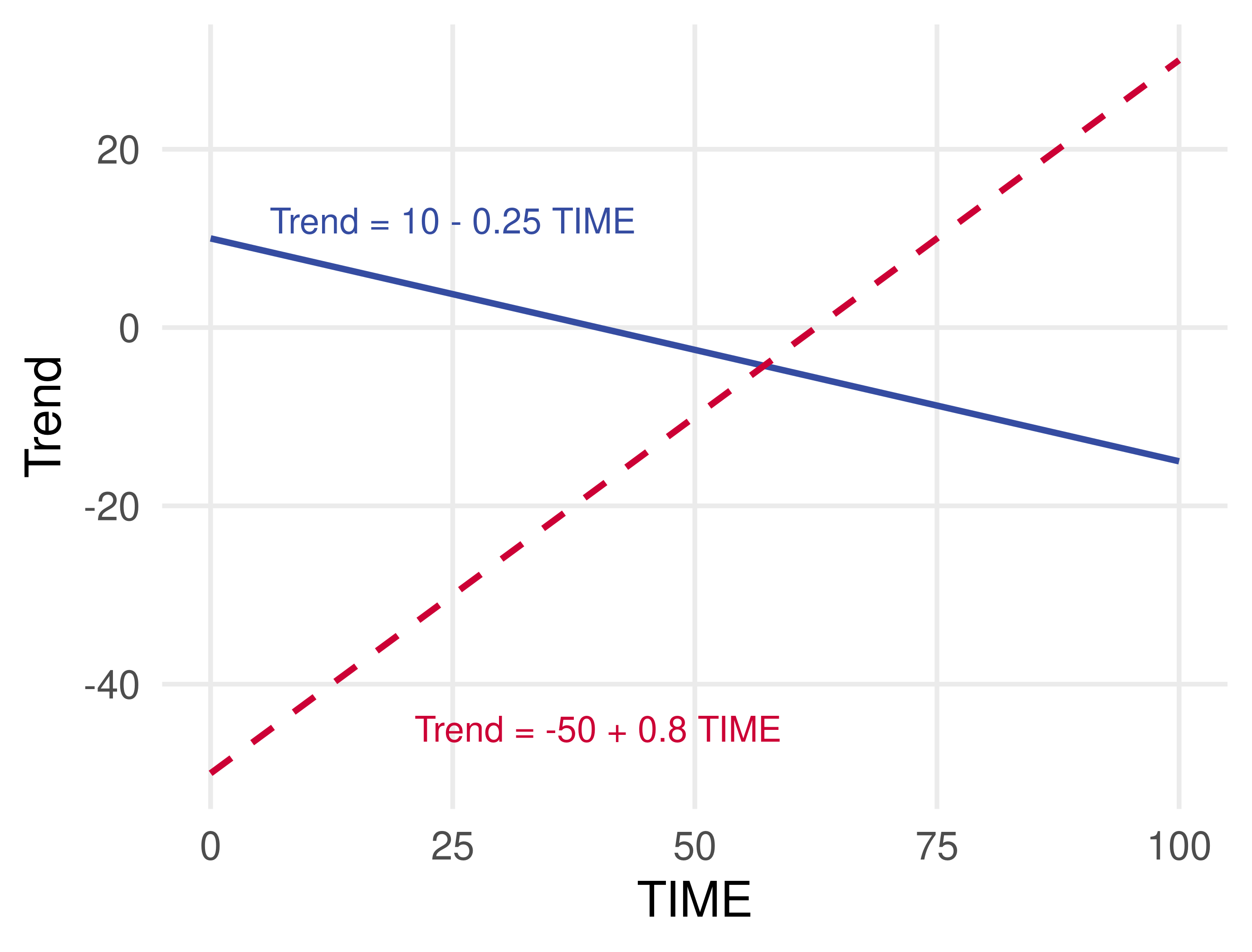
Sometimes a series rises or falls like a straight line:
T_t = \beta_0 + \beta_1\, TIME_t .
TIME_t = t: equal to 1 in the first period, 2 in the second, T in the last. An artificial regressor, so TIME_{T+h} = T + h is known today.
\beta_0: the trend at t = 0. \beta_1: the slope, the change per period. Larger |\beta_1|, steeper trend.
Quadratic trend
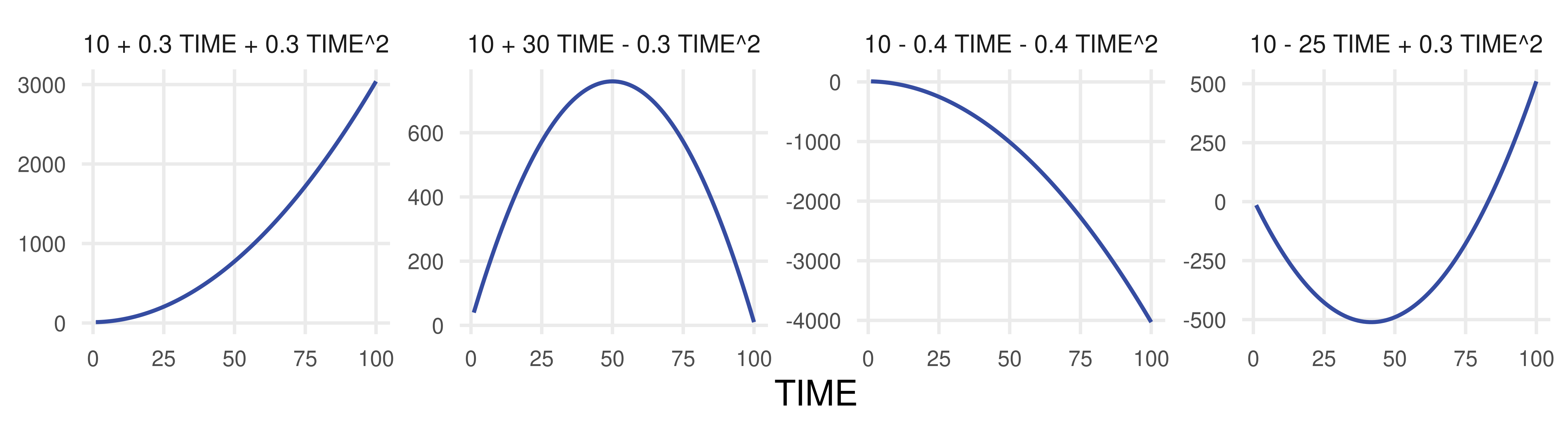
Trends need not be linear, but it needs to be smooth. A quadratic function of time captures a variable that grows at an increasing or decreasing rate:
Left to right: \beta_1, \beta_2 > 0, increasing at an increasing rate; \beta_1 > 0 > \beta_2, inverted U; \beta_1, \beta_2 < 0, decreasing; \beta_1 < 0 < \beta_2, U-shaped. Linear trend is the case \beta_2 = 0. In practice these are local approximations: one rarely sees a whole U.
Exponential trend
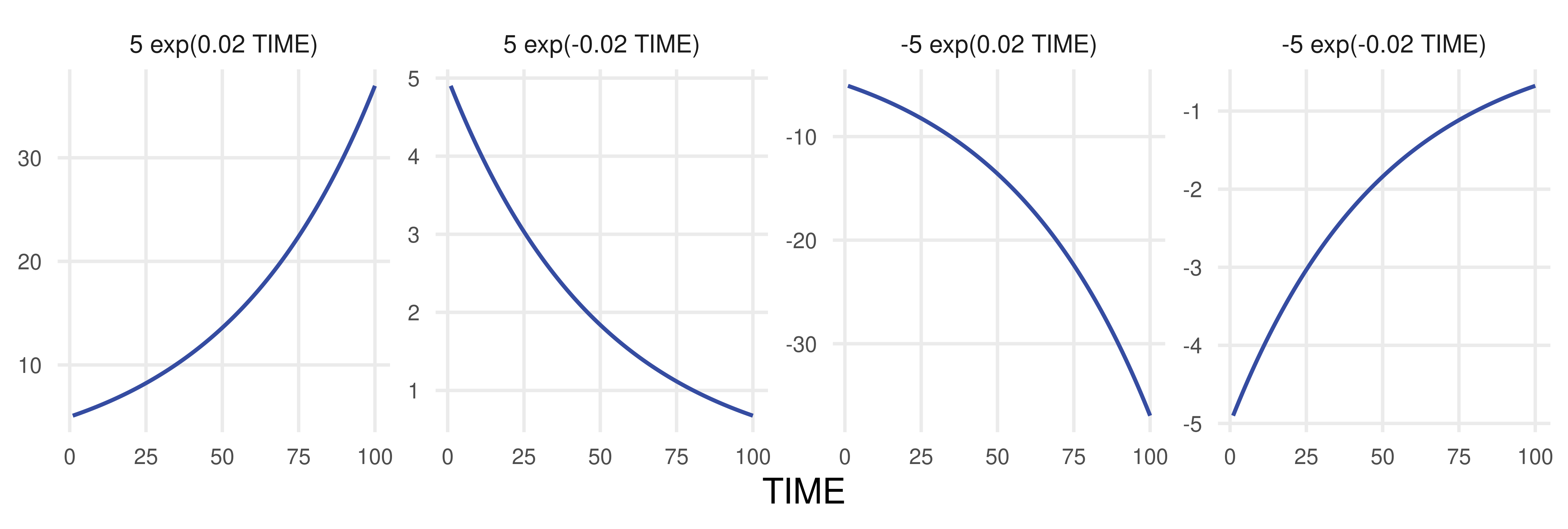
Many economic series grow at a roughly constant rate, say three percent a year. Constant growth at rate \beta_1 means
Nonlinear in levels, linear in logarithms: exponential or log-linear trend.
Logarithms are natural logarithms throughout. Recall from Lecture 5 why we took logs of liquor sales: proportional movements become additive.
Quadratic or exponential?
Both bend. Both can increase or decrease at an increasing or decreasing rate. Are they the same thing?
No. A quadratic and an exponential are different curves, and a series that is well approximated by one may be poorly approximated by the other.
Neither is “better” in general. Which fits a particular series is an empirical matter, settled by estimating both and comparing. We do that next.
Estimating and forecasting trends
Estimation by OLS
Create TIME = (1, 2, \ldots, T) and TIME^2 = (1, 4, \ldots, T^2), then run a regression. In Diebold’s shorthand (c denotes an intercept):
Trend
Regression
In R
linear
y \to c,\ TIME
lm(y ~ TIME)
quadratic
y \to c,\ TIME,\ TIME^2
lm(y ~ TIME + I(TIME^2))
exponential, in logs
\ln y \to c,\ TIME
lm(log(y) ~ TIME)
The first two are ordinary OLS regressions and need no comment.
The third is OLS too, but on \ln y: the intercept estimates \ln \beta_0, not \beta_0, and the fitted values are fitted values of \ln y. Exponentiate both to get back to levels.
No closed form: the computer searches numerically over (\beta_0, \beta_1). This is nonlinear least squares (NLS).
NLS is a general method, linear ones included. For linear models OLS is exact and instant, so use OLS.
Some forecasting models are intrinsically nonlinear and NLS is applicable.
Even here, where logs linearize the model, NLS in levels has a payoff: the AIC and SIC of the exponential trend become comparable with those of the linear and quadratic trends, which are in levels too.
“Argmin” is the argument that minimizes. Numerical search tries many candidate values, so it is slower than OLS and can stop at a local rather than the global minimum. Good starting values, from the log regression for instance, matter.
Point forecasts
At time T we hold \{y_1, \ldots, y_T\} and want y_{T+h}. The linear trend model holds at every date, in particular at T+h:
TIME_{T+h} = T + h. Known today. That is the whole point of a deterministic regressor.
\varepsilon_{T+h}: not known. Replace it by its optimal forecast given the time-T information set \Omega_T. For iid zero-mean noise that forecast is 0.
The subscript “T+h, T” reads: a forecast ofT+h, made atT. The hats make it operational. Quadratic and exponential trends: identical steps.
Choosing among trend models: AIC and SIC
Fit improves with every parameter; out-of-sample accuracy need not (Lecture 4: each parameter costs about \sigma^2 / T). Information criteria charge for parameters explicitly:
with k the number of estimated coefficients. Smaller is better. The first term rewards fit, the second penalizes size; SIC’s penalty is the heavier one whenever T > e^2 \approx 7.4, so SIC leans toward parsimony.
fit_stats <-function(m) { e <-residuals(m); y <-fitted(m) +residuals(m) T <-length(e); k <-length(coef(m)); ssr <-sum(e^2)c(R2 =1- ssr /sum((y -mean(y))^2), SER =sqrt(ssr / (T - k)),DW =sum(diff(e)^2) / ssr,AIC =log(ssr / T) +2* k / T, SIC =log(ssr / T) + k *log(T) / T)}
Only compare models with the same dependent variable on the same sample: y and \ln y are not comparable. Diebold writes AIC = e^{2k/T} SSR/T and SIC = T^{k/T} SSR/T; those are the exponentials of the versions above, so the rankings coincide. DW is the Durbin-Watson statistic, explained on the next slides.
Application: US retail sales
The retail sales data
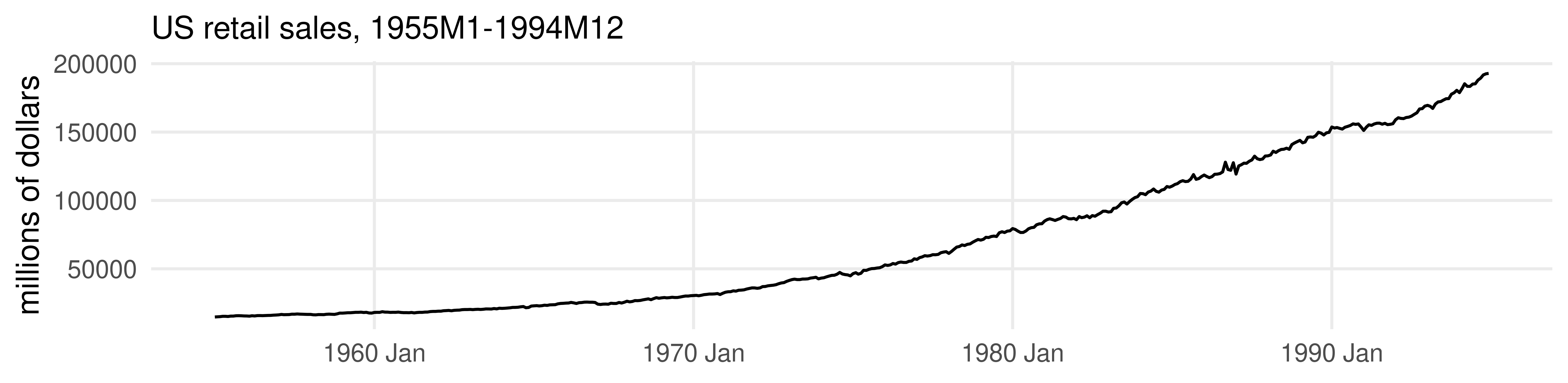
US retail sales, monthly, millions of current dollars, seasonally adjusted, 1955M1 to 1994M12. We estimate on 1955M1 to 1993M12 (T = 468) and hold out 1994 to check the forecasts.
“Seasonally adjusted”: a statistical agency removed the seasonal variation first. A clear nonlinear trend, and not much else.
Linear trend
lin <-lm(Sales ~ TIME, data = est)round(coef(summary(lin)), 4)
##                Estimate Std. Error  t value Pr(>|t|)
## (Intercept) -16391.2480  1469.1767 -11.1568        0
## TIME           349.7731     5.4287  64.4307        0
round(fit_stats(lin), 4)
##         R2        SER         DW        AIC        SIC
##     0.8991 15866.1151     0.0047    19.3481    19.3659
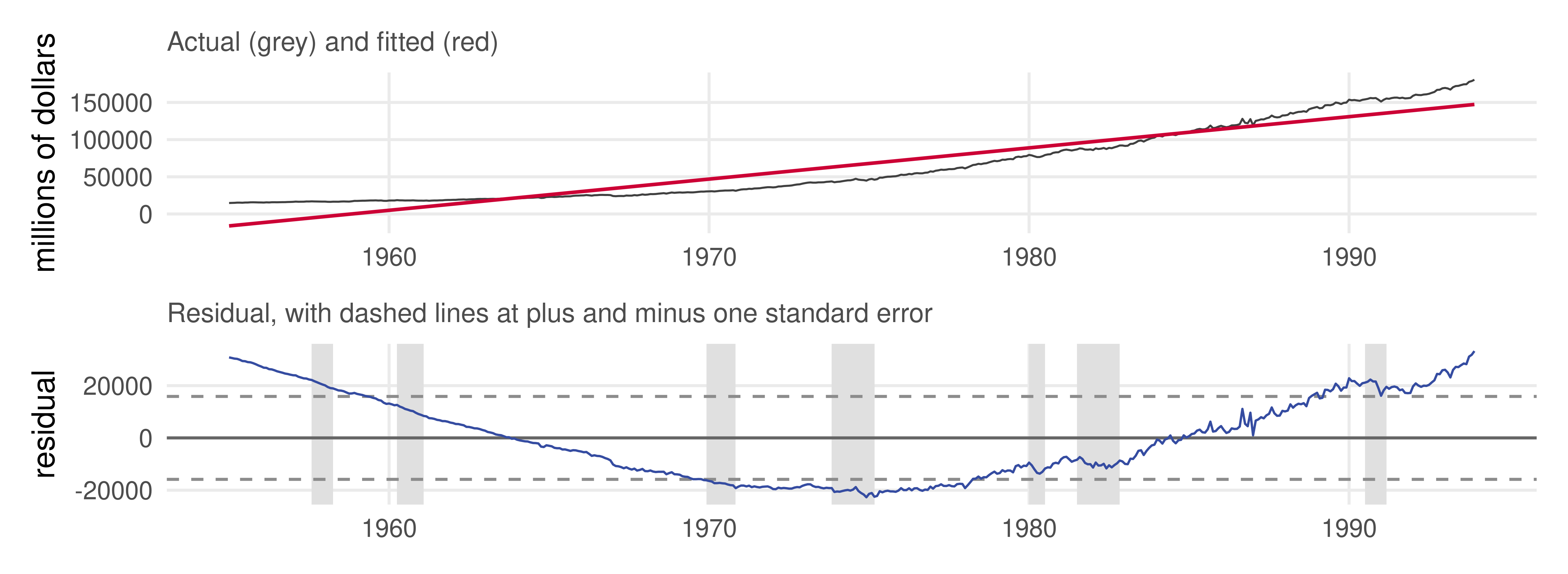
The trend is “highly significant”: t = 64. R^2 = 0.90. It looks like a fine model.
The Durbin-Watson statistic is DW = \sum_t (e_t - e_{t-1})^2 / \sum_t e_t^2. It is near 2 when residuals are uncorrelated and near 0 when each residual is close to the last one. Here it is 0.005: the residuals are extremely positively serially correlated. Something is wrong. Look at the picture.
Serial correlation makes OLS standard errors and t-statistics untrustworthy; Newey-West (HAC) standard errors repair them. AIC and SIC remain valid. Later lectures model the correlation instead of just correcting for it.
Linear trend: residual plot
The residuals are first all positive, then all negative for fifteen years, then all positive. The linear trend is simply inadequate: the true trend is curved.
Shaded bands are NBER recessions. fit_plot(), fc_plot() and dec_year() are short ggplot helpers defined in the source of these slides.
Quadratic trend
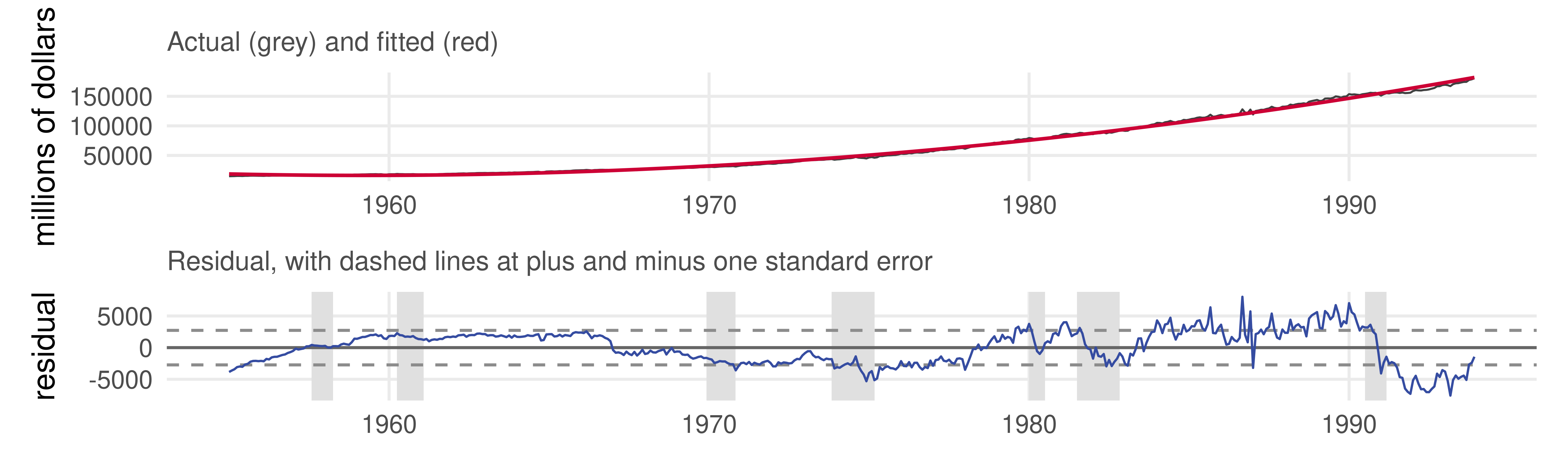
quad <-lm(Sales ~ TIME +I(TIME^2), data = est)round(coef(quad), 4); round(fit_stats(quad), 4)
## (Intercept)        TIME   I(TIME^2)
##  18708.7003    -98.3113      0.9554
##        R2       SER        DW       AIC       SIC
##    0.9970 2728.2050    0.1511   15.8292   15.8558
R^2 is now 0.997 and the fitted curve tracks the series. The residuals are still persistent (DW = 0.15) but they are now recession-sized dips and boom-sized bumps: business cycle, not trend. No trend model can explain those.
Log-linear trend
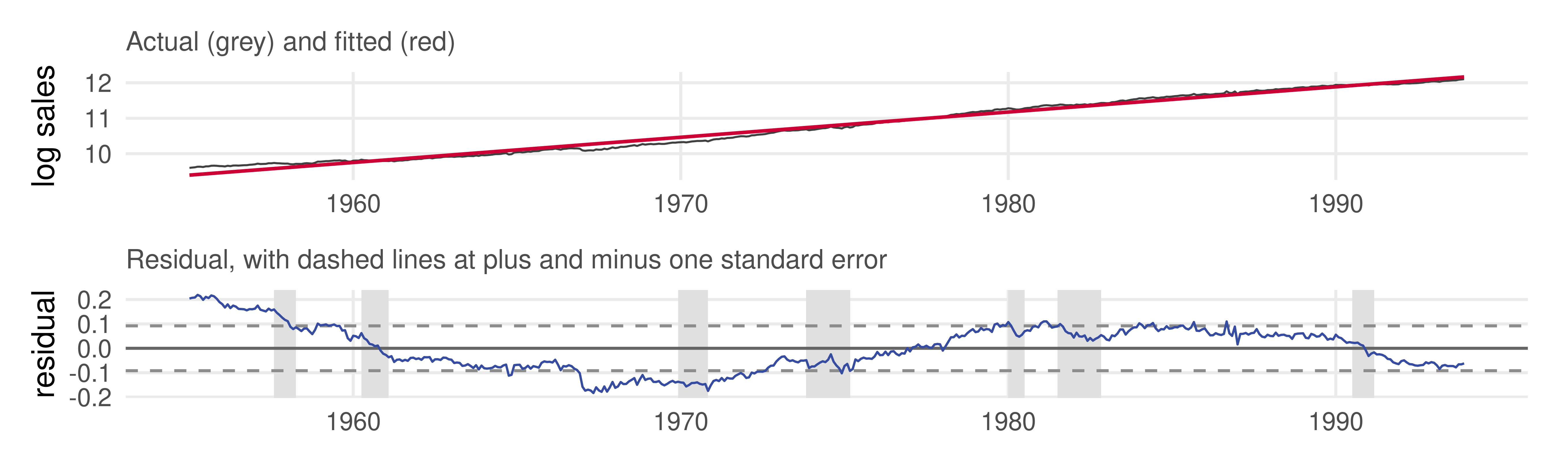
loglin <-lm(log(Sales) ~ TIME, data = est)round(coef(loglin), 5); round(fit_stats(loglin), 4)
## (Intercept)        TIME
##     9.38997     0.00593
##      R2     SER      DW     AIC     SIC
##  0.9871  0.0919  0.0199 -4.7703 -4.7526
Growth of 0.59% per month, about 7.4% per year in nominal terms. The fit looks good. But every statistic here is in logs, so none of them can be compared with the linear and quadratic models in levels.
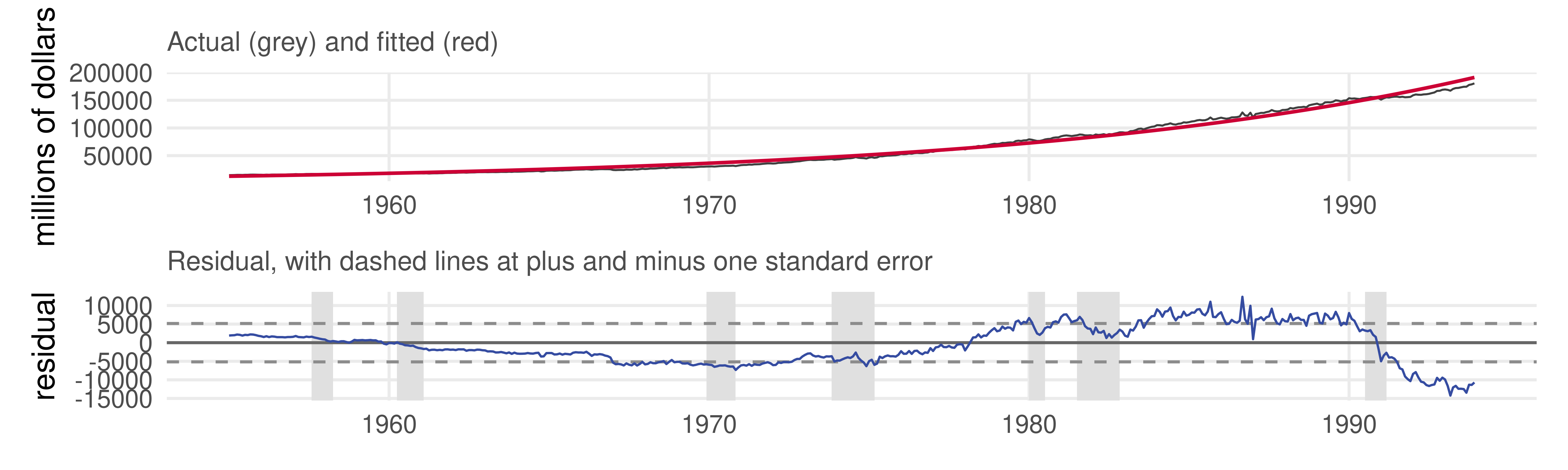
##        R2       SER        DW       AIC       SIC
##    0.9893 5168.3697    0.0423   17.1049   17.1226
Now in levels, so comparable: better than the linear trend, worse than the quadratic. The book’s EViews output reports \hat\beta_0 = 11968; it stopped after one iteration, while nls() continues to a lower sum of squares. Same conclusion either way.
Both criteria rank the linear trend last: nonlinearity matters.
Both favor the quadratic trend, even after paying for its extra parameter. So we use it.
The log-linear row is a trap. Its AIC is “the smallest” only because \ln y is a different variable on a different scale. Never compare criteria across dependent variables.
Informal impressions, in-sample fit, and the criteria all agree here. They will not always. When they disagree, the criteria win: they are the only ones that price parsimony.
Forecasting 1994 with the quadratic trend
new <-data.frame(TIME =469:480) # 1994M1 to 1994M12fc <-predict(quad, newdata = new); s <-sigma(quad)qfc <-data.frame(t =dec_year(yearmonth("1994 Jan") +0:11),point = fc, lower = fc -1.96* s, upper = fc +1.96* s)round(head(qfc, 3), 2)
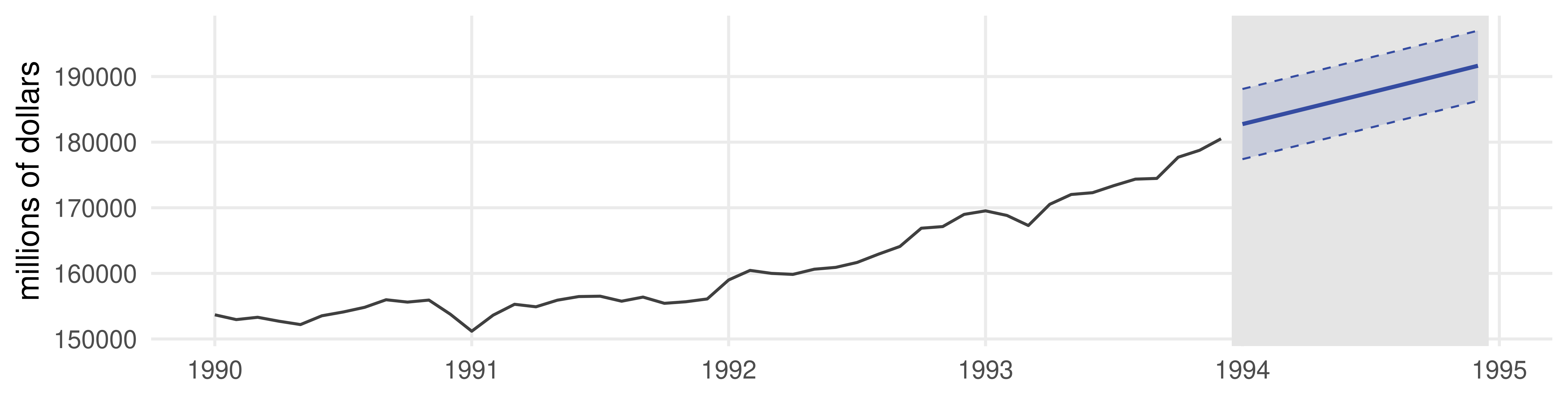
History 1990M1 to 1993M12, point forecast and 95% interval for 1994. The point forecasts look reasonable. The interval has constant width because the model treats deviations from trend as noise, which the residual plot said they are not.
Forecasting 1994 with the quadratic trend (cont.)
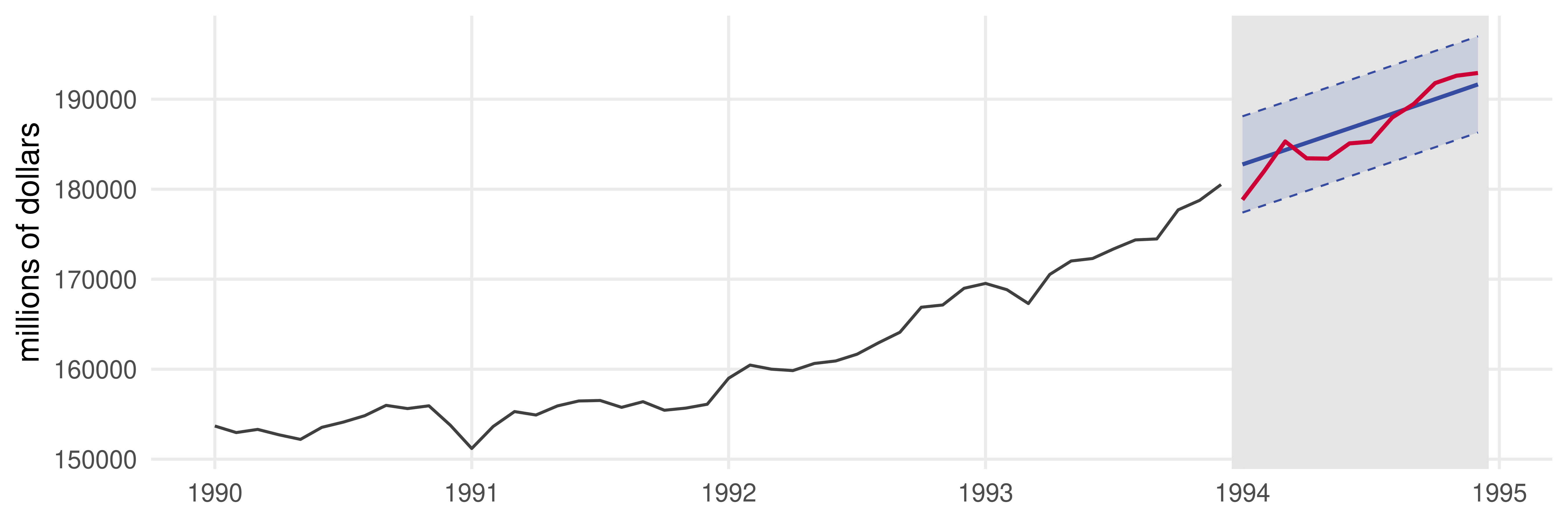
Now add the realization (red). The forecast is quite good: the realization hugs the extrapolated trend, and all twelve months fall inside the 95% interval.
The linear trend, for comparison
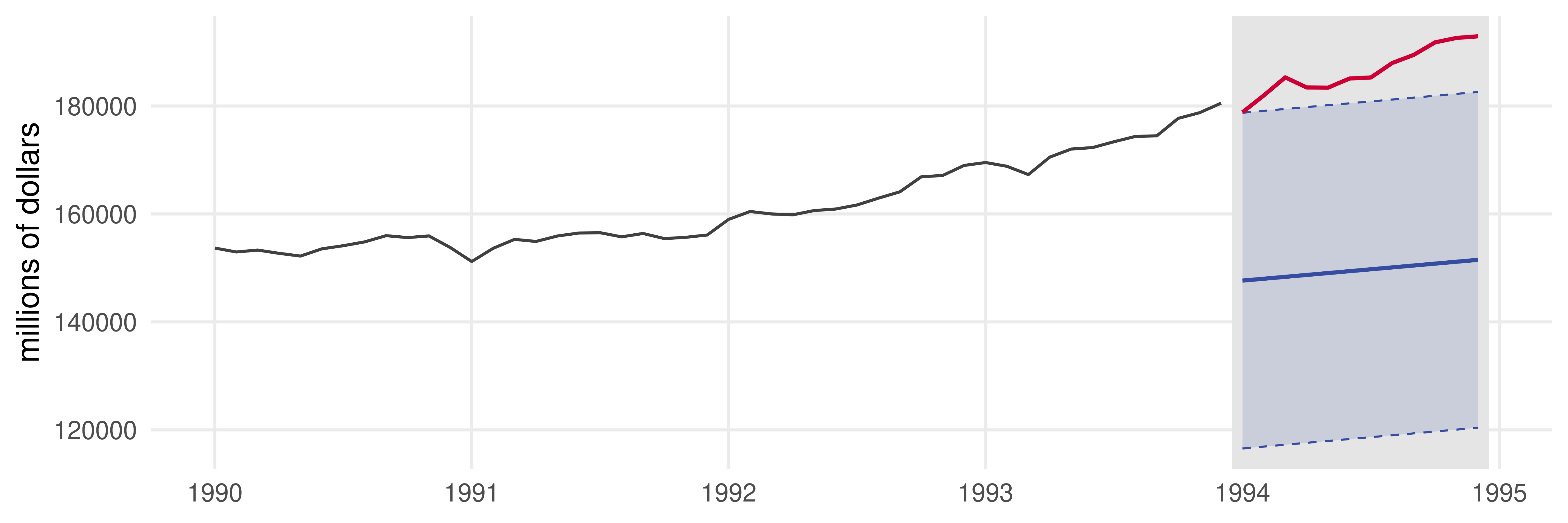
The point forecast is below the last observation, because by 1993 the linear trend sits far under the sample path. The interval is enormous (\hat\sigma = 15{,}866 versus 2{,}728) and still misses every month.
Forecasts are computed as if the model were the true process. A poor approximation to the trend gives confidently wrong forecasts, and the interval will not save you.
Seasonal models
Seasonality
y_t = S_t + \varepsilon_t
Seasonality is a pattern that repeats every year, produced by technologies, preferences and institutions that are tied to the calendar.
Technology. Anything that involves the weather: agriculture, construction, energy.
Preferences. Vacation travel every summer raises both the price and the quantity of gasoline every July.
Institutions. Holidays. Retail purchases explode every December (the liquor series of Lecture 5).
You might guess that only a few obviously seasonal series are affected. On the contrary: seasonality is pervasive in business and economic data, and it is often the largest source of variation within a year.
Seasonality is impossible, and therefore a non-issue, in data recorded once a year or less often.
Seasonal dummies
Let s be the number of observations per year: s = 4 for quarterly data, 12 for monthly, 52 for weekly. Create s dummies, one per season. With s = 4,
an intercept that changes with the season and repeats every year. The \gamma_i are the seasonal factors; together they are the seasonal pattern.
No seasonality means \gamma_1 = \cdots = \gamma_s: drop the dummies and keep an ordinary intercept. Like TIME, the dummies are known at every future date: deterministic seasonality is perfectly predictable.
Estimation
Regress y on the full set of dummies, with no intercept:
y \to D_1, \ldots, D_s .
Why no intercept: the dummies sum to 1 at every date, so an intercept plus all s dummies is perfectly collinear (the dummy variable trap, Lecture 3). Keep the intercept and drop one dummy instead, and you get the same fit with a different parameterization: an intercept plus s - 1differences from the omitted season.
Blend trend and seasonality by adding TIME and TIME^2: \ y \to TIME,\ TIME^2,\ D_1, \ldots, D_s.
d <- d |>mutate(m =factor(month(Month), labels = month.abb)) # the season, as a factorlm(y ~0+ m, data = d) # 0 removes the intercept; m expands to 12 dummieslm(y ~0+ TIME +I(TIME^2) + m, data = d) # quadratic trend plus seasonal dummies
When the intercept is dropped, R’s summary() reports an R^2 measured about zero instead of about the mean, and it comes out absurdly high. fit_stats() uses the centered version.
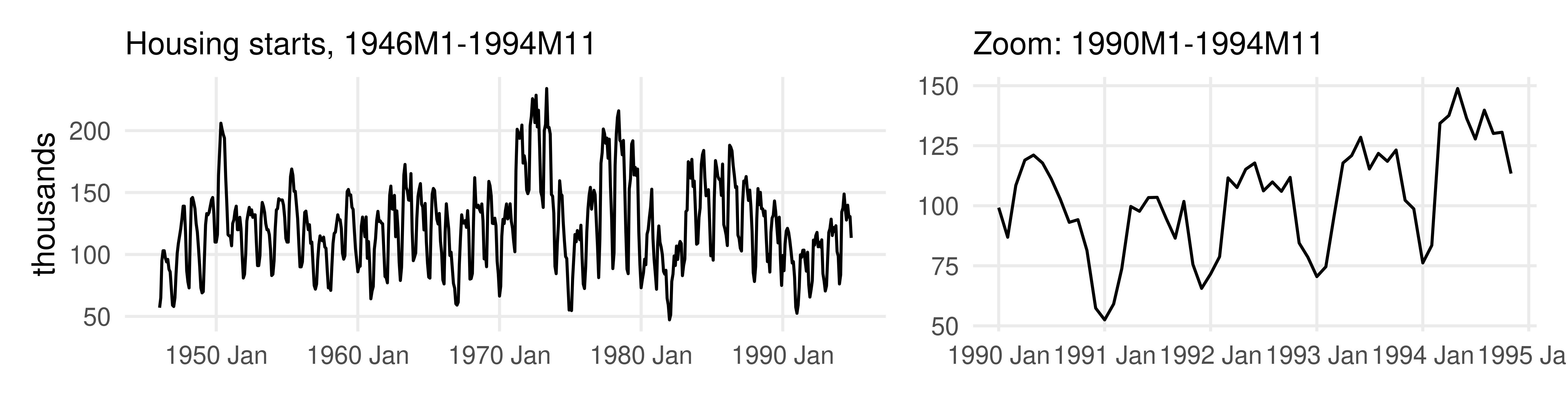
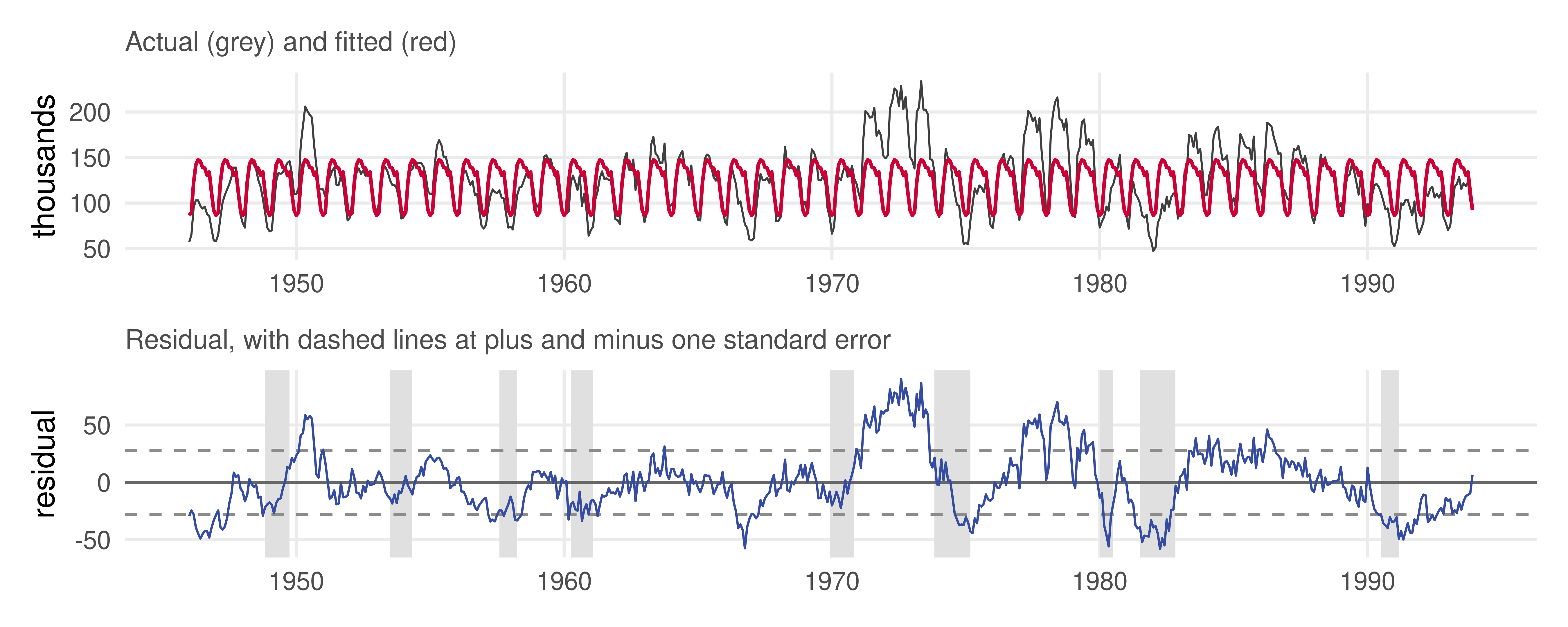
Housing starts is an economic indicator that reflects the number of privately owned new houses (technically housing units) on which construction has been started in a given period. Houses are started in spring so that they finish before winter: the same within-year shape every year, and no trend. A pure seasonal model, then.
Twelve dummies
seas <-lm(Starts ~0+ m, data = hest)round(coef(summary(seas)), 3)
##     R2    SER     DW    AIC    SIC
##  0.384 27.914  0.154  6.679  6.770
R^2 = 0.38: the twelve dummies explain more than a third of the variation. The rest is largely cyclical (DW = 0.15, a measure of serial correlation (will be explained in the next lecture)), which the model was not built to capture. Every standard error is the same because every month has 48 observations: \hat\sigma / \sqrt{48}.
Residual plot
The fitted values go through the same twelve numbers every year; nothing else is in the model, yet that rigid pattern picks up a lot. What it misses is serially correlated: dips in the residuals in the recessions of 1975, 1980, 1982 and 1990 (shaded), peaks in booms.
Estimated seasonal factors
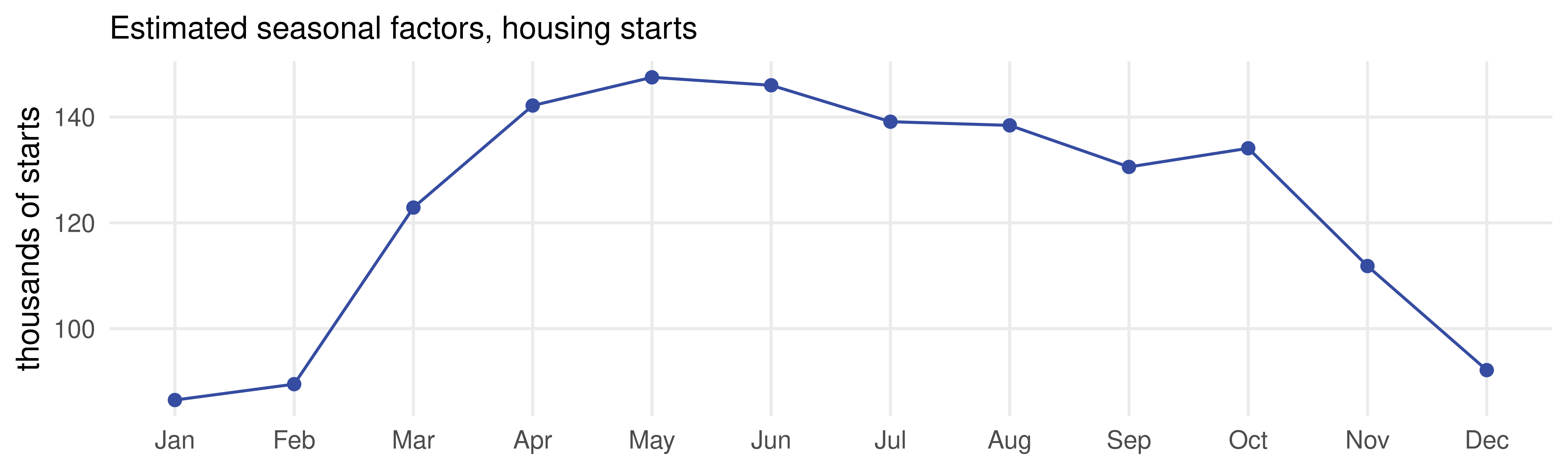
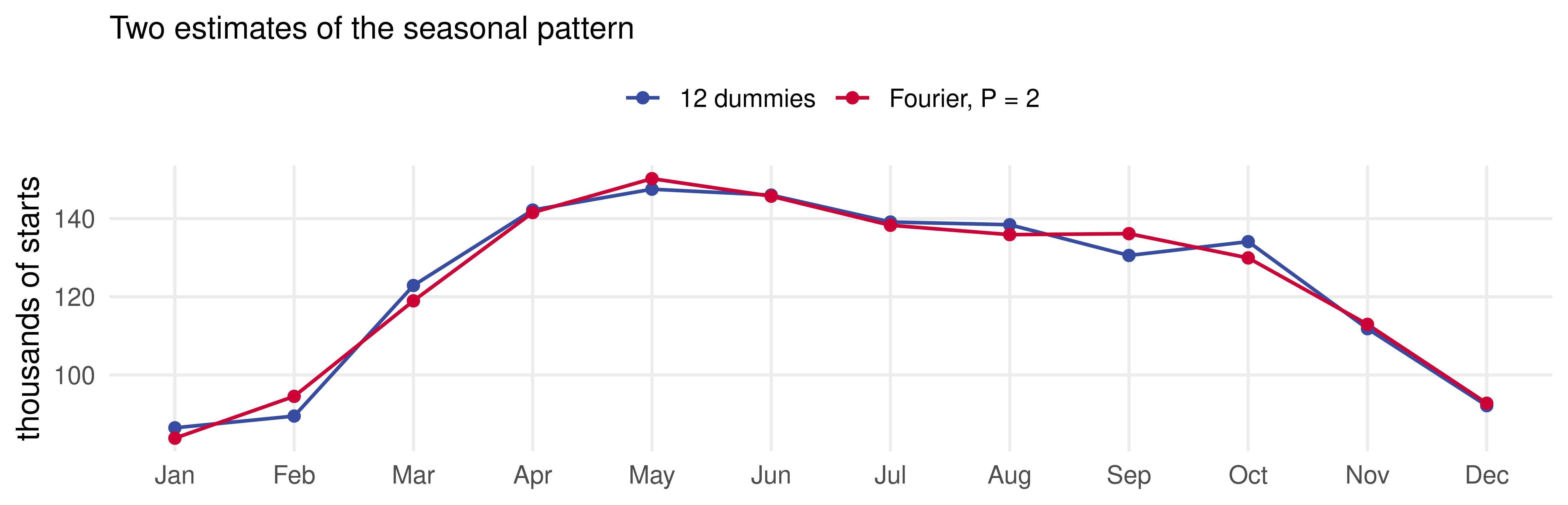
Very low in January and February, a quick rise to a peak in May, then a slow decline until October and an abrupt drop in November and December.
With only dummies on the right-hand side, each \hat\gamma_i is simply the sample mean of season i. Regression on seasonal dummies is monthly averages with standard errors attached, and the factors are exactly the blue lines of gg_subseries() from Lecture 5.
Forecasting 1994
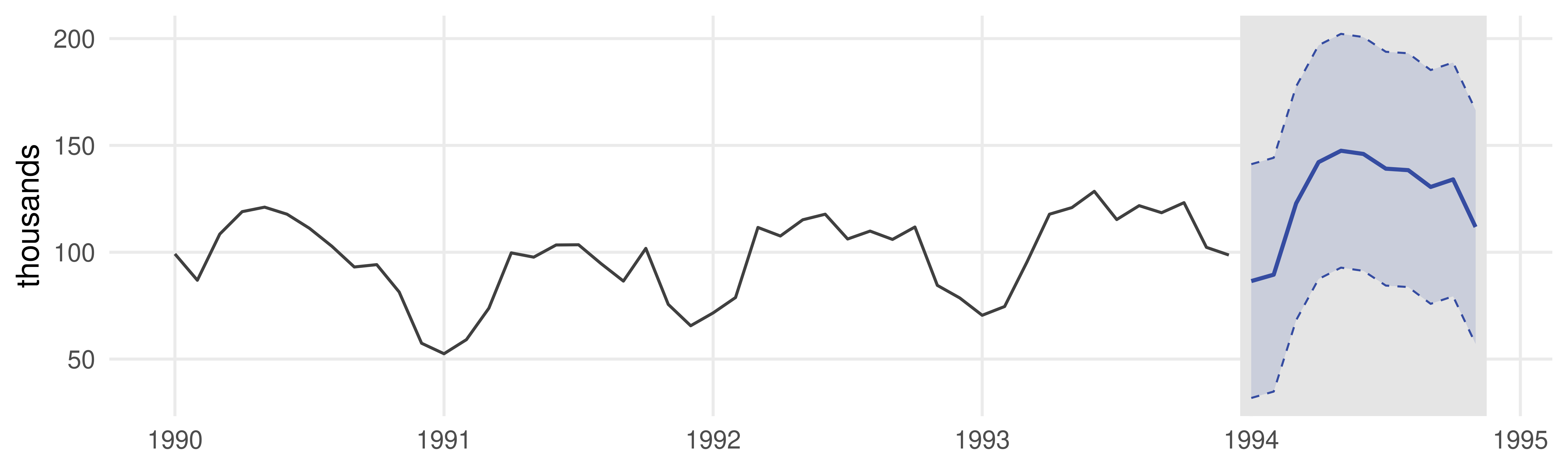
new <-data.frame(m =factor(month.abb[1:11], levels = month.abb)) # 1994M1 to 1994M11fc <-predict(seas, newdata = new); s <-sigma(seas)hfc <-data.frame(t =dec_year(yearmonth("1994 Jan") +0:10),point = fc, lower = fc -1.96* s, upper = fc +1.96* s)
The forecast is the seasonal pattern itself, and it looks reasonable. The interval is wide, because the seasonal factors account for only a third of the variation in the series.
Forecasting 1994 (cont.)
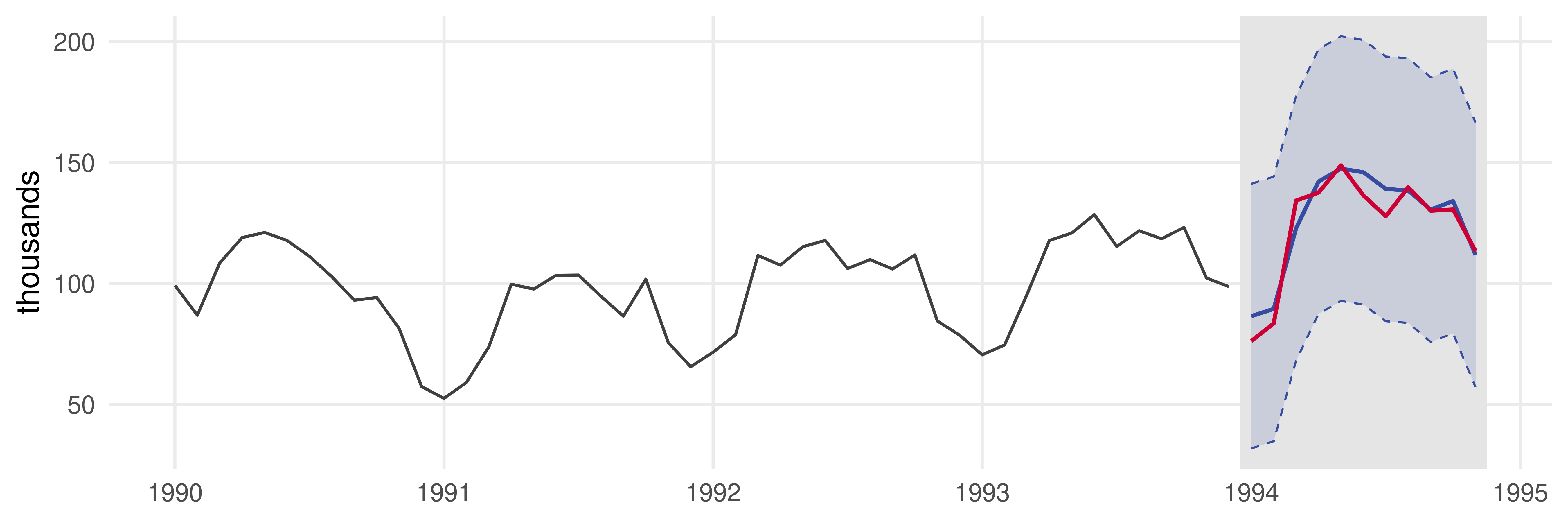
With the realization added: the forecast is close throughout, and the realization stays well inside the 95% interval. The model did its job; the job was to predict the season, and the season is predictable.
Trend and seasonality together
Liquor sales, again
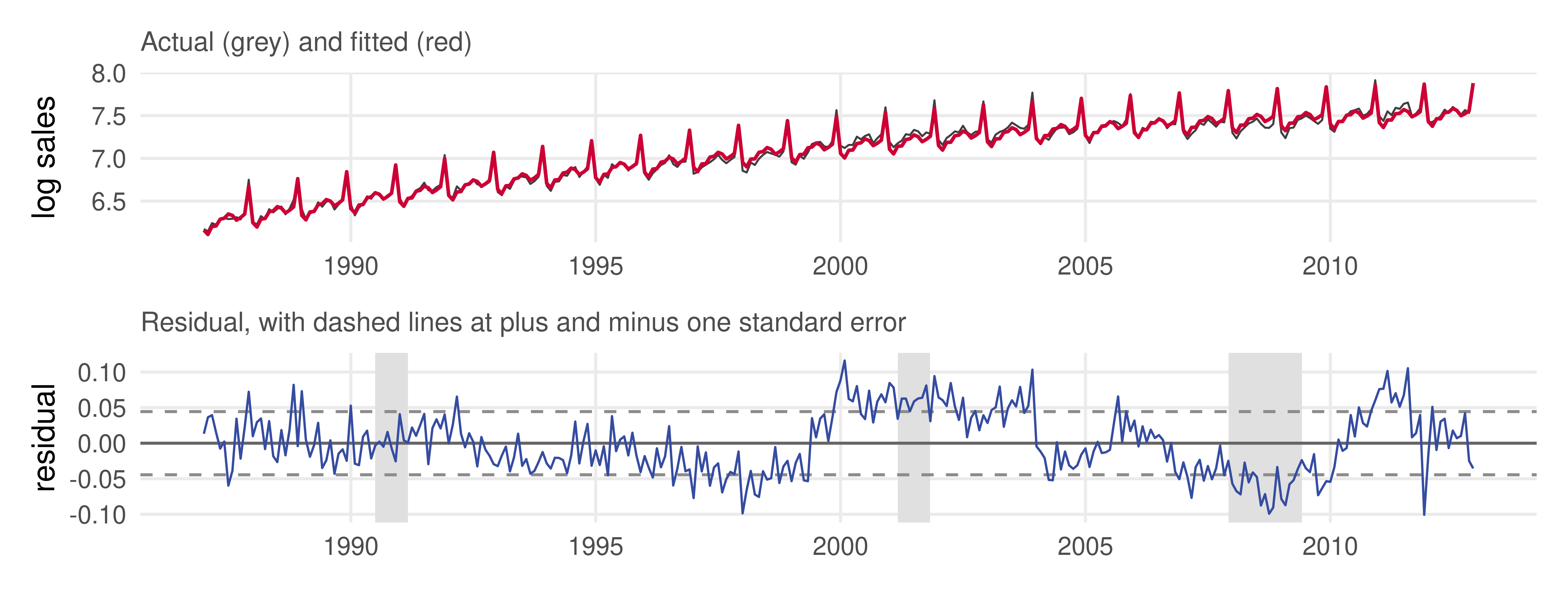
Lecture 5’s liquor series has both components, and its seasonal swings grow with the level, so we work in logs. Log-quadratic trend plus twelve seasonal dummies, estimated on 1987M1 to 2012M12 with 2013 and 2014 held out for evaluation:
##      R2     SER      DW     AIC     SIC
##  0.9884  0.0444  0.6438 -6.1842 -6.0162
Fitted values and residuals
Trend and seasonal together explain 99% of the variation in log sales. The December factor sits about 0.37 above the average of the other eleven: December sales are e^{0.37} \approx 1.45 times a typical month. The residuals are persistent (DW = 0.64) and recession-shaped. The cycle, again.
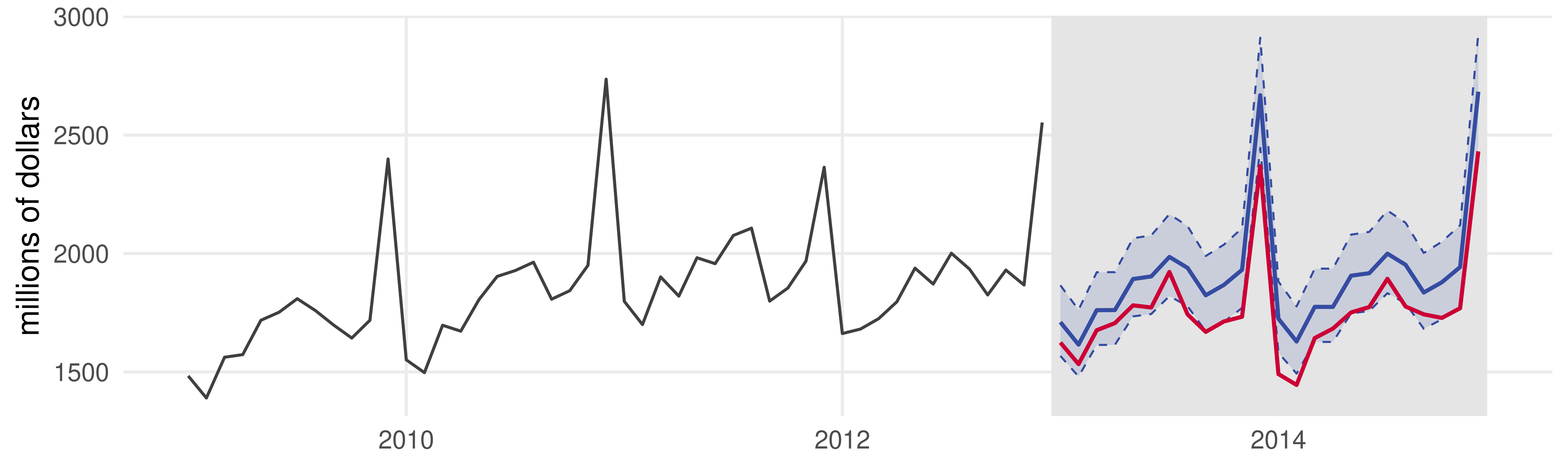
Out of sample: 2013 and 2014
new <-data.frame(TIME =313:336, m =factor(rep(month.abb, 2), levels = month.abb))p <-predict(lq, newdata = new); s <-sigma(lq) # forecasts of log saleslfc <-data.frame(t =dec_year(yearmonth("2013 Jan") +0:23),point =exp(p), lower =exp(p -1.96* s), upper =exp(p +1.96* s))
Forecast in logs, then exponentiate the point forecast and both interval endpoints. The interval is asymmetric in levels. The two Decembers are forecast almost exactly; the forecast is a little high in 2013, when growth slowed more than the quadratic expected.
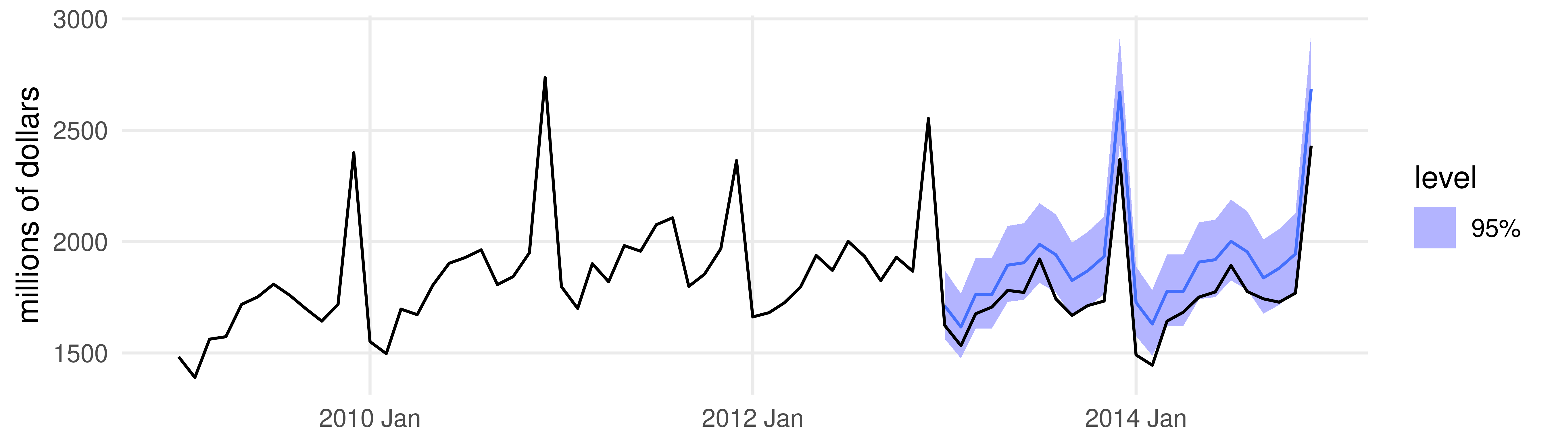
The same in three lines with fable
TSLM() builds TIME and the dummies for you, and forecast() returns the distribution, back-transformed to levels.
fit <- liquor |>filter(year(Month) <=2012) |>model(TSLM(log(Sales) ~trend() +I(trend()^2) +season()))fit |>forecast(h =24) |>autoplot(liquor |>filter(year(Month) >=2009), level =95) +labs(y ="millions of dollars", x =NULL)
One difference from the hand version: fable’s point forecast is the mean of the back-transformed distribution, ours was the median e^{\hat p}; with \hat\sigma = 0.044 they differ by 0.1%. The interval here also includes parameter uncertainty.
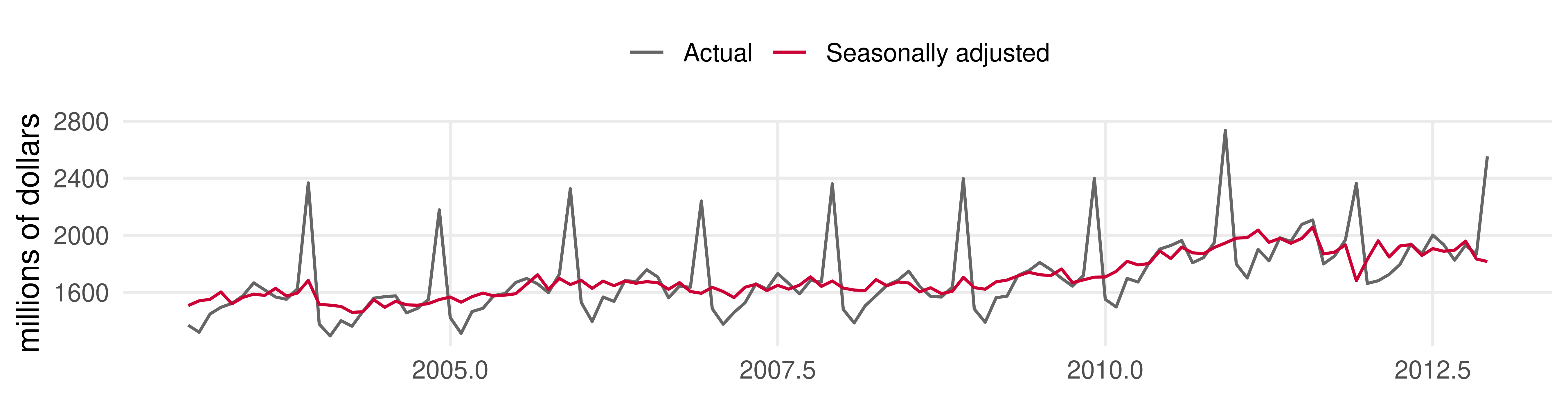
Seasonal adjustment
Removing seasonality is called seasonal adjustment. With dummies it is a subtraction: take out the estimated seasonal factors, centered, and keep the rest.
g <-coef(lq)[paste0("m", month.abb)] # the twelve factorssa <- lest |>mutate(SA =exp(log(Sales) - (g[as.integer(m)] -mean(g))))
Macroeconomists usually want the nonseasonal movements, and official series come pre-adjusted (Census X-13ARIMA-SEATS). Business forecasters usually want all the variation: if seasonality is most of what moves your series, the last thing to do is discard it.
Fourier seasonality
Dummies are one basis for a periodic pattern. Sines and cosines are another:
Smooth, and parsimonious: 2P coefficients instead of s. With P = s/2 the two bases are identical; with small P you get a smoothed seasonal. Choose P with AIC or SIC. Indispensable for daily data, where s = 365 dummies is not appealing.
hest <- hest |>mutate(t =row_number())four <-lm(Starts ~cos(2*pi*t/12) +sin(2*pi*t/12) +cos(4*pi*t/12) +sin(4*pi*t/12), data = hest)round(rbind(`12 dummies`=fit_stats(seas), `Fourier, P = 2`=fit_stats(four)), 3)
##                   R2    SER    DW   AIC   SIC
## 12 dummies     0.384 27.914 0.154 6.679 6.770
## Fourier, P = 2 0.376 27.913 0.193 6.667 6.705
Five parameters instead of twelve, nearly the same fit, and both criteria prefer Fourier. In fable: fourier(K = 2).
Fourier seasonality (cont.)
Two harmonics reproduce the rise, the plateau and the fall; what they smooth away is the small kink at the September to October step, which is well within a standard error anyway.
Detrending: the Hodrick-Prescott filter
Detrending: Hodrick-Prescott filter
The polynomial trends above are global: one curve for the whole sample, which is why the retail-sales residuals swung for decades. The Hodrick-Prescott (HP) filter is a curve fitting procedure proposed by Hodrick and Prescott (1997) to estimate the trend path of a series, letting the trend bend locally.
y_t is decomposed into a trend component and a cyclical component y_t = y_t^\star + c_t
The HP filter: \min_{y_1^\star, y_2^\star, \ldots, y_T^\star}\left[\sum_{t=1}^T \left(y_t - y_t^\star\right)^2 + \lambda \sum_{t=2}^{T-1}\left(\Delta^2 y_{t+1}^\star\right)^2\right] where \lambda is a tuning parameter: it penalizes changes in the trend’s slope, \Delta^2 y^\star_{t+1} = (y^\star_{t+1} - y^\star_t) - (y^\star_t - y^\star_{t-1}).
Conventional choice: \lambda = 1600 for quarterly data, \lambda = 100 for annual data.
Ravn and Uhlig (2002) argue for \lambda = 6.25 with annual and \lambda = 129{,}600 with monthly data.
Two limits and a closed form
\lambda = 0: no penalty, y^\star_t = y_t. The “trend” is the data.
\lambda \to \infty: slope changes are forbidden, so y^\star is a straight line: the linear trend fitted by OLS, as in Section 3.
In between, a smooth trend that follows the data as closely as the smoothness budget allows.
The objective is quadratic in y^\star, so the solution is linear in the data:
hp_filter <-function(y, lambda) { T <-length(y); D <-diff(diag(T), differences =2) # second-difference matrix trend <-as.numeric(solve(diag(T) + lambda *crossprod(D), y))list(trend = trend, cycle = y - trend)}data("IRE", package ="bHP") # log Irish GDP, annual 1981-2016; used again belowmax(abs(hp_filter(IRE, 100)$trend - bHP::BoostedHP(IRE, lambda =100, iter =FALSE)$trend))
## [1] 1.634248e-13
US real GDP, \lambda = 1600
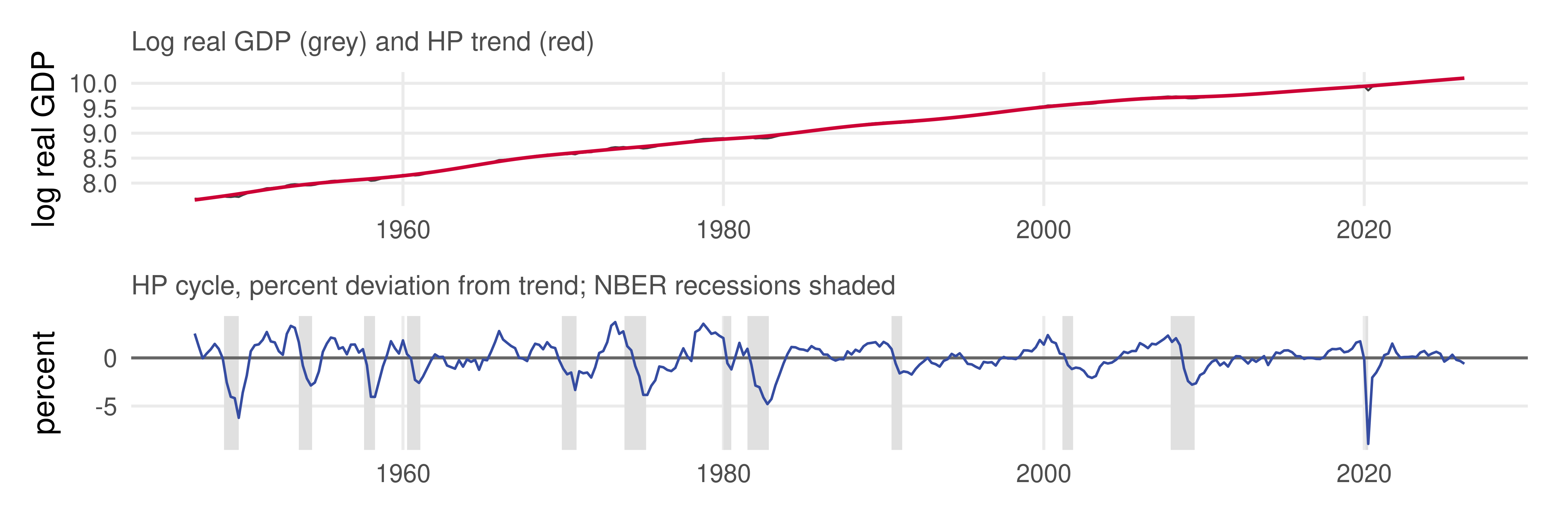
gdp <-read.csv("data/GDPC1.csv") |>mutate(Quarter =yearquarter(as.Date(Date)), y =log(GDPC1),t =year(Quarter) + (quarter(Quarter) -1) /4)hp <-hp_filter(gdp$y, lambda =1600)
Quarterly, 1947Q1 to 2026Q2, from FRED (series GDPC1). The cycle turns down in every shaded recession; a typical swing is \pm 2\%, and 2020 is off that scale.
Boosted HP filter
Phillips, P. C. B., & Shi, Z. (2021). Boosting: Why you can use the HP filter. International Economic Review, 62(2), 521-570.
When the series is very persistent, one pass of the HP filter leaves some trend behind in c_t. Iterate the HP filter to fully remove the trend: filter the cycle again, add what it finds to the trend, and stop when the cycle is stationary (ADF test) or when the BIC stops improving. With S = (I_T + \lambda D'D)^{-1}, after m passes the cycle is \hat c^{(m)} = (I_T - S)^m y.
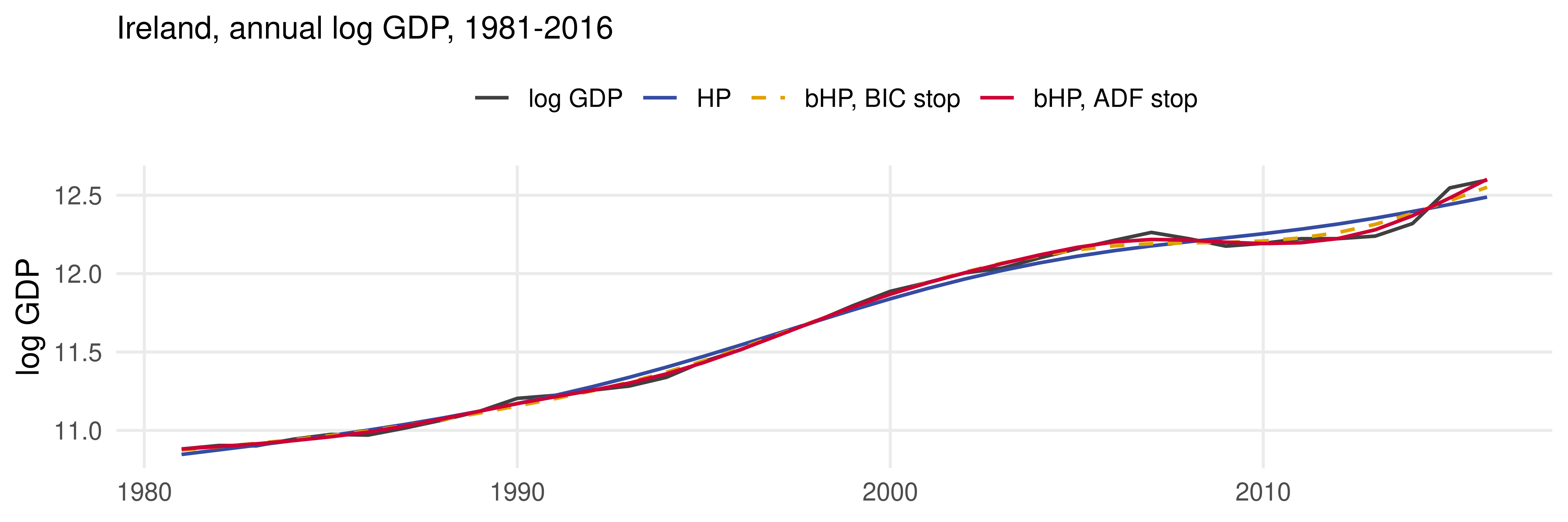
lam <-100# tuning parameter for the annual data# raw HP filterbx_HP <- bHP::BoostedHP(IRE, lambda = lam, iter =FALSE)# stopping stands for the condition of the terminal of iteration# by BICbx_BIC <- bHP::BoostedHP(IRE, lambda = lam, iter =TRUE, stopping ="BIC")# by ADFbx_ADF <- bHP::BoostedHP(IRE, lambda = lam, iter =TRUE, stopping ="adf")c(BIC = bx_BIC$iter_num, ADF = bx_ADF$iter_num) # passes until the stopping rule fires
## BIC ADF
##   5  19
What boosting changes
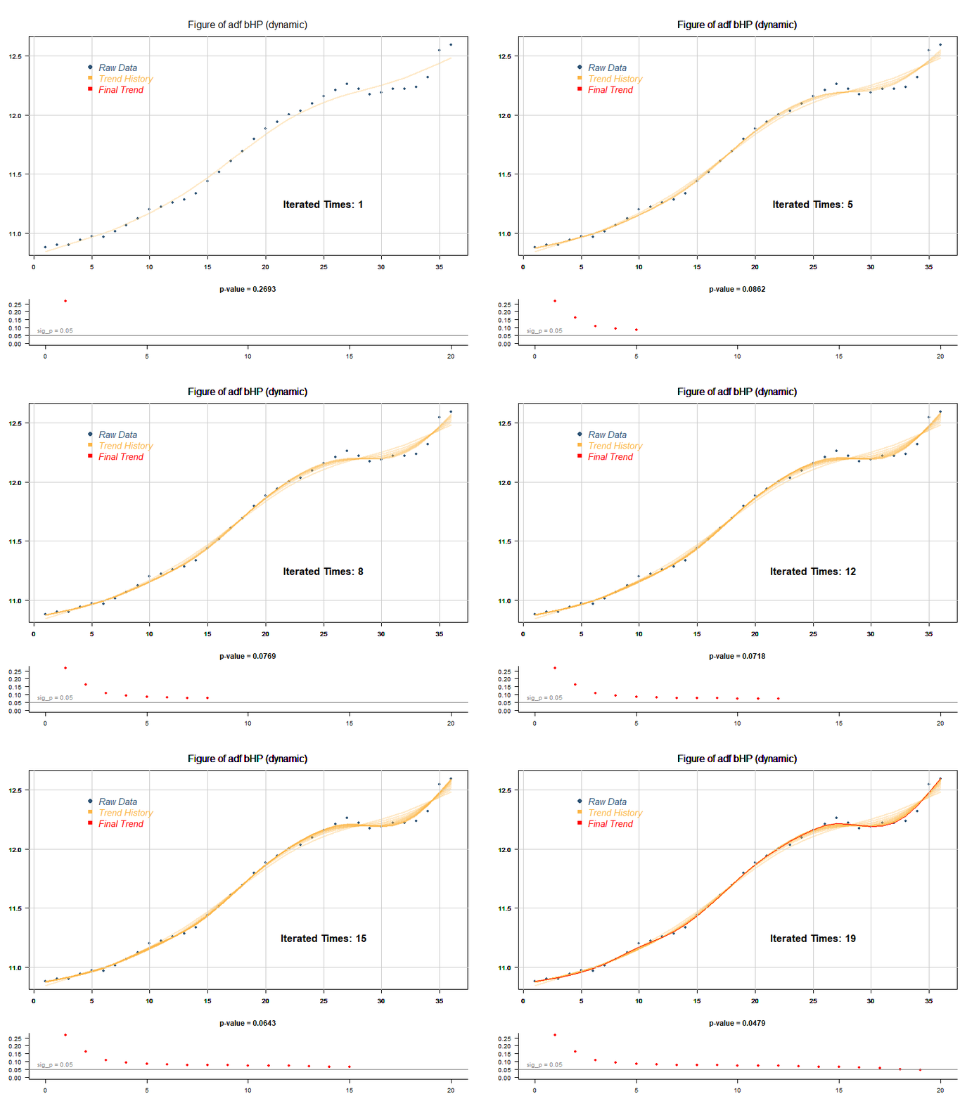
One HP pass (\lambda = 100) leaves a trend that ignores the 2008 collapse and the 2015 jump, so both end up in the “cycle”. Boosting bends the trend toward the data: five passes under BIC, nineteen under the ADF rule, at which point the remaining cycle is stationary at the 5% level.
Boosted HP filter: the iterations
# Dynamic demonstration: draws the trend after each pass (run in your console)plot(bx_ADF, iteration_location ="upright", interval_t =0.8)
A caution for forecasters
The HP trend at date t is a weighted average of the data on both sides of t. That is fine in the middle of the sample. At the end, where a forecaster lives, there is no future data to average over: the last trend values are the least reliable, and they get revised as new observations arrive.
So the filter is a tool for describing history, not for extrapolating it. Hamilton (2018) makes the case at length under the title “Why you should never use the Hodrick-Prescott filter”; Phillips and Shi’s reply is titled “Why you can use the HP filter”.
To forecast a trending series, model the trend and the cycle explicitly. That is what the rest of the course does.
What to take away
Deterministic regressors dodge the FRV problem. TIME and seasonal dummies are known at every future date, so trend and seasonal forecasts are fitted values extended forward.
Fit linear, quadratic and exponential trends by OLS or NLS, choose with AIC or SIC in levels, then extrapolate. A bad trend model gives confidently wrong forecasts.
Seasonal dummies are seasonal averages with standard errors; they blend with a trend in one regression; Fourier terms are the parsimonious alternative.
The residuals of every model today were persistent. That is the cycle, and it is next.
The HP filter is a local, two-sided trend estimator: excellent for describing history, unreliable exactly where a forecaster needs it.
R cheat sheet
library(fpp3)d <- d |>mutate(TIME =row_number(), m =factor(month(Month), labels = month.abb))# ---- trends -------------------------------------------------------------------lm(y ~ TIME, data = d); lm(y ~ TIME +I(TIME^2), data = d); lm(log(y) ~ TIME, data = d)nls(y ~ b0 *exp(b1 * TIME), data = d, start =list(b0 =100, b1 =0.01)) # exponential, in levels# ---- seasonals ----------------------------------------------------------------lm(y ~0+ m, data = d) # 12 dummies = monthly meanslm(y ~0+ TIME +I(TIME^2) + m, data = d) # trend and seasonal togetherlm(y ~cos(2*pi*t/12) +sin(2*pi*t/12), data = d) # Fourier, P = 1# ---- forecasts ----------------------------------------------------------------predict(fit, newdata =data.frame(TIME = T +1:h, m = ...)) # point forecastssigma(fit) # SER: interval is point +- 1.96 * sigmafit_stats(fit) # R2, SER, DW, AIC, SIC (defined in these slides)model(d, TSLM(log(y) ~trend() +I(trend()^2) +season())) |>forecast(h =24) # fable# ---- detrending ---------------------------------------------------------------hp_filter(y, lambda =1600) # trend and cycle (defined in these slides)bHP::BoostedHP(y, lambda =1600, iter =TRUE, stopping ="adf") # boosted HP
References
Additional resources
Textbooks
Diebold, F.X. Forecasting in Economics, Business, Finance and Beyond, Chapter 5. The retail sales and housing starts applications come from Elements of Forecasting, 4th edition, Chapters 5 and 6.
Hodrick, R.J. and Prescott, E.C. (1997), “Postwar U.S. Business Cycles: An Empirical Investigation,” Journal of Money, Credit and Banking, 29, 1–16.
Ravn, M.O. and Uhlig, H. (2002), “On Adjusting the Hodrick-Prescott Filter for the Frequency of Observations,” Review of Economics and Statistics, 84, 371–376.
Hamilton, J.D. (2018), “Why You Should Never Use the Hodrick-Prescott Filter,” Review of Economics and Statistics, 100, 831–843.
Phillips, P.C.B. and Shi, Z. (2021), “Boosting: Why You Can Use the HP Filter,” International Economic Review, 62, 521–570. R package bHP.
Data
data/retail_sales.csv, data/housing_starts.csv — from the Elements of Forecasting companion files, converted from EViews.
data/liquor_sales.csv — as in Lecture 5. data/GDPC1.csv — real GDP from FRED, downloaded September 2026.
IRE — annual log GDP of Ireland, 1981–2016, shipped with bHP.