e <- seq(-3, 3, length.out = 400)
linlin <- function(e, a) ifelse(e >= 0, a * e, (a - 1) * e)

par(mfrow = c(1, 3), mar = c(4, 4, 2.5, 1))
plot(e, e^2,  type = "l", lwd = 2, main = "quadratic", xlab = "error e", ylab = "L(e)")
plot(e, abs(e), type = "l", lwd = 2, main = "absolute", xlab = "error e", ylab = "")
plot(e, linlin(e, 0.8), type = "l", lwd = 2, col = "#cc0035",
main = "lin-lin, alpha = 0.8", xlab = "error e", ylab = "")ECON 4354 / 6354 Forecasting
Lecture 4: The Basics of Forecasting
Zhan Gao
15 September 2026
From estimation to prediction
Lecture 3 gave us the machinery: OLS, its assumptions, its standard errors.
But machinery answers only the last question in a forecasting project.
Before any of it, someone has to decide what to forecast, how to state the forecast, how far ahead, using what information, and how much complexity to buy.
Today: the six questions that come before the model.
Roadmap
Sections 1–6 are Diebold’s six considerations basic to successful forecasting (Elements of Forecasting, Chapter 3). Section 0 and Section 7 come from Hyndman and Athanasopoulos, Chapter 1.
Groundwork
Forecasting is old, and hard
“Stock prices have reached what looks like a permanently high plateau.”
— Irving Fisher, Yale economist, 16 October 1929
“There is no reason anyone would want a computer in their home.”
— Ken Olsen, founder of Digital Equipment Corporation, 1977
“Why did nobody notice it?”
— Elizabeth II, on the financial crisis, London School of Economics, November 2008
The often-quoted “world market for maybe five computers,” attributed to IBM’s Thomas Watson in 1943, appears to be apocryphal. Be careful with famous quotations; it is an occupational hazard of this subject.
Forecasting, goals, and planning
Three things that are routinely confused inside organizations:
- Forecasting is predicting the future as accurately as possible, given all the information available — including the knowledge that you cannot control the outcome.
- Goals are what you would like to happen. A goal is not a forecast. There is no guarantee a goal is achievable, and often no plan for how to get there.
- Planning is the response to forecasts and goals: the actions that close the gap between what you expect and what you want.
A forecast that has been adjusted to match a goal is not a forecast.
Planning horizons
| Horizon | Typical questions | Typical tools |
|---|---|---|
| Short-term (days to weeks) | staff rosters, inventory, production runs | detailed, high-frequency models |
| Medium-term (months to ~2 years) | raw materials, hiring, equipment | the bulk of this course |
| Long-term (years) | market entry, capacity, strategy | scenarios, judgement, structural models |
The horizon is not a detail. It changes the data frequency, the model, the loss function, and how much of the answer is judgement rather than statistics.
What can be forecast?
Not everything. Accuracy depends on four things:
- How well we understand the factors that contribute to the outcome.
- How much data are available.
- Whether the future will resemble the past.
- Whether the forecast itself can affect the thing being forecast.
The forecaster’s first job is to tell the difference between what can be forecast and what cannot.
Two extremes
| Electricity demand tomorrow | The $/€ exchange rate tomorrow | |
|---|---|---|
| Do we understand the drivers? | yes: temperature, day of week, holidays | barely |
| Do we have data? | decades, half-hourly | decades, by the second |
| Will the future resemble the past? | yes, over a day | not through a crisis |
| Does the forecast move the outcome? | no | yes |
Short-horizon electricity demand is forecast to within a couple of percent. Nobody beats the random walk for tomorrow’s exchange rate — and if you could, publishing the forecast would destroy it.
Meese and Rogoff (1983) is the classic reference for the second column. It is still, uncomfortably, roughly true.
Forecasts that change the outcome
Two ways a published forecast contaminates its own target:
- Self-fulfilling. Forecast a bank run; depositors queue; the run happens. Forecast a currency depreciation; traders sell; it depreciates.
- Self-defeating. Forecast a traffic jam on I-75; drivers reroute; there is no jam. Forecast a shortage; the firm restocks; no shortage.
This is not a nuisance to be assumed away. It is why financial-market forecasting is hard in principle, and it is the forecasting cousin of the Lucas critique and Goodhart’s law.
There is always an irreducible floor
Even a perfect model with infinite data leaves error. Split next period’s value:
Y_{T+1} \;=\; \underbrace{E(Y_{T+1} \mid \Omega_T)}_{\text{the best any model can do}} \;+\; \underbrace{\varepsilon_{T+1}}_{\text{unforecastable}}
From Lecture 3, the expected squared error of any forecast \hat Y_{T+1} built from \Omega_T decomposes as
E\big[(Y_{T+1} - \hat Y_{T+1})^2\big] = \underbrace{\sigma^2_\varepsilon}_{\text{irreducible}} + \underbrace{\text{bias}^2 + \text{variance}}_{\text{ours to reduce}}
A “bad” forecast with a big \sigma^2_\varepsilon may be the best possible one. Judge forecasts against a benchmark, never against zero error.
The six questions
- Decision environment and loss function. What decision does this guide, and what does an error cost?
- Forecast object. What exactly are we forecasting?
- Forecast statement. A number, a range, or a distribution?
- Forecast horizon. How far ahead?
- Information set. Built from what?
- Methods and complexity. How elaborate should the model be?
Answer these six before you open R.
1. The decision environment and loss function
Forecasts are made to guide decisions
A stylized problem. You run a distributor and must set inventory now, for a sales period whose demand you will only learn later.
- Demand turns out high and you built inventory: good.
- Demand turns out low and you cut inventory: good.
- The two off-diagonal cases cost you money.
Every decision problem has a loss structure. The forecast inherits it.
Symmetric loss
Table 1. Loss ($) by decision and outcome.
| Demand high | Demand low | |
|---|---|---|
| Build inventory | 0 | 10,000 |
| Cut inventory | 10,000 | 0 |
Both mistakes cost the same. This is often a reasonable approximation, and it is mathematically convenient — which is why it is the default everywhere, including in this course.
Asymmetric loss
Table 2. Same problem, more realistic costs.
| Demand high | Demand low | |
|---|---|---|
| Build inventory | 0 | 10,000 |
| Cut inventory | 20,000 | 0 |
Running out of stock loses the sale and the customer; carrying stock only ties up capital. Under-forecasting now costs twice as much as over-forecasting.
Nothing about the statistics has changed. What changed is which forecast you should report.
From decisions to forecast errors
The decision loss induces a loss over forecasts, because the forecast picks the decision. Let
e_{T+h\mid T} \;=\; \underbrace{Y_{T+h}}_{\text{realization}} - \underbrace{\hat Y_{T+h\mid T}}_{\text{forecast made at } T}
We work with loss functions of the form L(e): the cost depends only on the size and sign of the error. We require
- L(0) = 0 — a perfect forecast is free.
- L is continuous — nearly identical errors cost nearly the same.
- L is increasing on each side of the origin — bigger errors hurt more.
Beyond these three, anything goes.
Three loss functions
Quadratic (squared-error) loss
L(e) = e^2
Symmetric; penalizes large errors at an increasing rate.
Absolute-error loss
L(e) = |e|
Symmetric; penalizes at a constant rate, so it cares less about outliers.
Lin-lin (asymmetric absolute) loss, for \alpha \in (0,1):
L_\alpha(e) = \begin{cases} \alpha\, e, & e \ge 0 \quad (\text{we under-forecast})\\[2pt] (\alpha - 1)\, e, & e < 0 \quad (\text{we over-forecast}) \end{cases}
\alpha = 1/2 gives absolute loss (up to a factor of 2). \alpha > 1/2 makes under-forecasting the expensive mistake.
Three loss functions, plotted
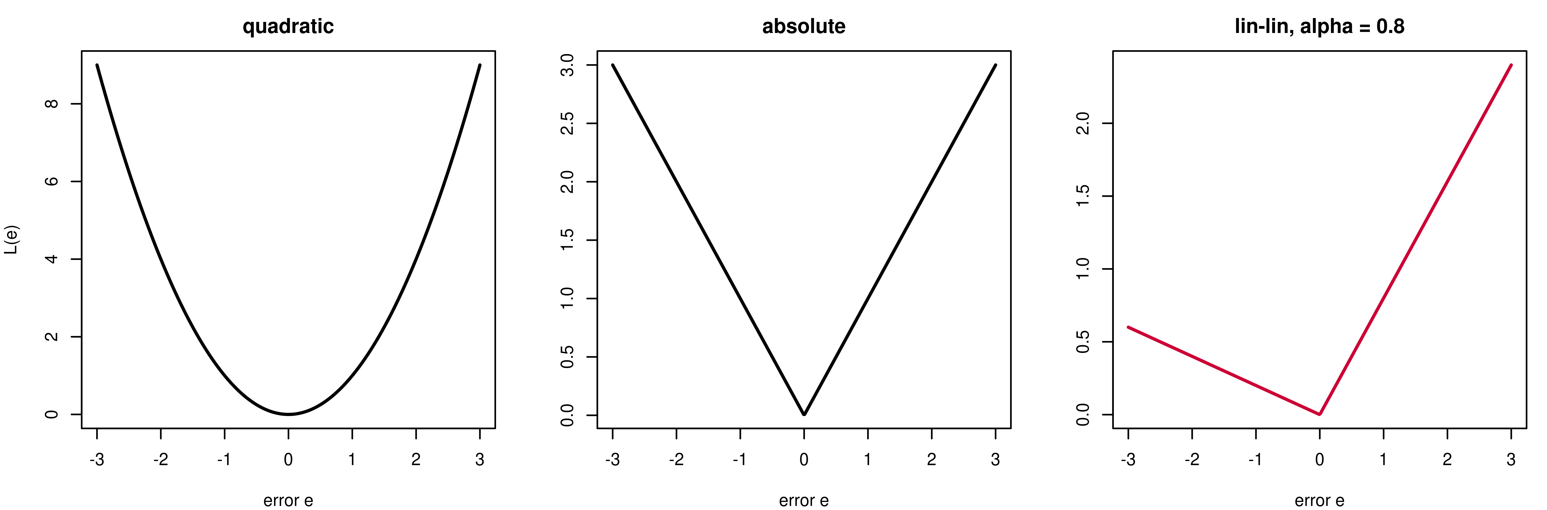
In the third panel, under-forecasting (right of zero) is four times as costly as over-forecasting.
Loss that is not a function of the error alone
Sometimes even L(e) is too restrictive. In finance, interest often focuses on the direction of change:
L = \begin{cases} 0, & \text{if } \operatorname{sign}(\Delta \hat Y_{T+h\mid T}) = \operatorname{sign}(\Delta Y_{T+h})\\ 1, & \text{otherwise} \end{cases}
A forecast can be badly wrong in level and still perfect under this loss — and a forecast with tiny mean squared error can get the sign wrong half the time.
The loss function is a modelling choice, and it is yours to make.
What is an optimal forecast?
The forecast that minimizes expected loss, given the information available.
\hat Y_{T+h\mid T} \;=\; \arg\min_{f}\; E\big[\,L(Y_{T+h} - f) \;\big|\; \Omega_T\,\big]
Two things to notice.
- The expectation is conditional on \Omega_T: optimality is relative to what you know.
- The answer depends on L. Change the loss, change the forecast.
Squared-error loss picks out the conditional mean
Claim. If L(e) = e^2, the optimal forecast is \hat Y_{T+h\mid T} = E(Y_{T+h}\mid \Omega_T).
Proof. Write \mu = E(Y_{T+h}\mid\Omega_T) and add and subtract it:
E\big[(Y_{T+h} - f)^2 \mid \Omega_T\big] = E\big[(Y_{T+h} - \mu)^2 \mid \Omega_T\big] + (\mu - f)^2
The cross term vanishes because E[(Y_{T+h} - \mu)\mid\Omega_T] = 0 and (\mu - f) is known at time T. The first term does not involve f; the second is minimized at f = \mu. \;\blacksquare
This is the promise Lecture 3 made: a forecast is a conditional expectation — provided you have agreed to quadratic loss.
Other losses pick out other features
| Loss L(e) | Optimal forecast |
|---|---|
| e^2 | conditional mean E(Y_{T+h}\mid\Omega_T) |
| \lvert e \rvert | conditional median |
| lin-lin with weight \alpha | conditional \alpha-quantile |
For a symmetric predictive distribution the first two coincide, and the loss function does not matter much. For a skewed one — sales, claims, prices, durations — they can be far apart.
The lin-lin result is the one behind quantile regression, and it is why interval forecasts and asymmetric loss are the same subject viewed from two sides.
Seeing it: a skewed predictive density
Suppose the predictive distribution of next quarter’s sales is lognormal — a floor at zero, a long right tail.
mu <- 4.6; s <- 0.5                       # log sales ~ N(4.6, 0.5^2)
y  <- seq(20, 320, length.out = 600)
plot(y, dlnorm(y, mu, s), type = "l", lwd = 2, xlab = "sales next quarter",
     ylab = "density", yaxs = "i", ylim = c(0, 0.012))
abline(v = c(qlnorm(0.5, mu, s), exp(mu + s^2/2)),
       col = c("#354ca1", "#cc0035"), lwd = 2, lty = c(2, 1))
legend("topright", c("median", "mean"), col = c("#354ca1", "#cc0035"),
       lwd = 2, lty = c(2, 1), bty = "n")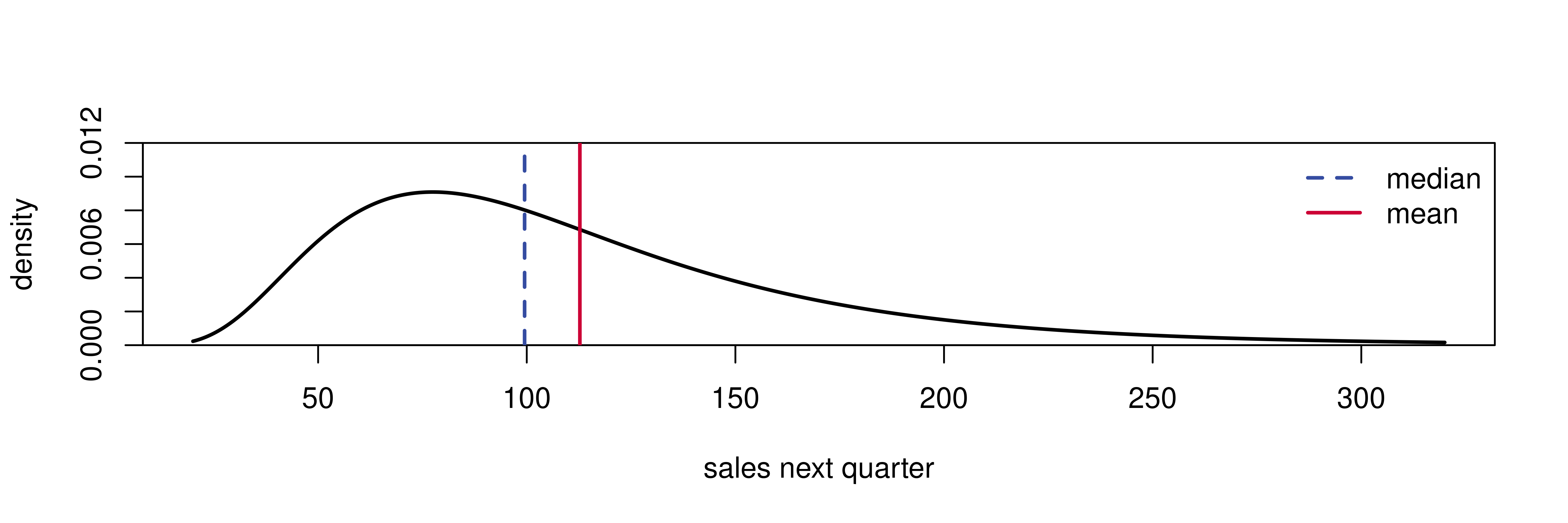
The loss function chooses the number
EL   <- function(f, L) integrate(function(y) L(y - f) * dlnorm(y, mu, s), 0, Inf)$value
best <- function(L) optimize(function(f) EL(f, L), interval = c(40, 260))$minimum
linlin <- function(a) function(e) ifelse(e >= 0, a * e, (a - 1) * e)

round(c(quadratic     = best(function(e) e^2),
        absolute      = best(abs),
        `lin-lin 0.75` = best(linlin(0.75)),
        `lin-lin 0.25` = best(linlin(0.25))), 1)
## quadratic absolute lin-lin 0.75 lin-lin 0.25
## 112.7 99.5 139.3 71.1## mean median q75 q25
## 112.7 99.5 139.4 71.0The numerical optima match the theory to the optimizer’s tolerance. One predictive distribution, four defensible point forecasts — differing by nearly a factor of two.
What to take away
- Loss is not a technicality bolted on at the evaluation stage. It defines what “best” means, and therefore what number you report.
- Quadratic loss is the default in this course. It is analytically convenient, it delivers the conditional mean, and it is often a decent approximation.
- But say so out loud, and check whether the decision it serves is really symmetric. A hospital forecasting bed demand and a retailer forecasting a perishable both know it is not.
2. The forecast object
Three kinds of forecast object
Event outcome. The event will certainly happen at a known time; the outcome is uncertain. Will the Fed chair be reconfirmed? Which firm wins the contract?
Event timing. The event will certainly happen and the outcome is known; the timing is uncertain. When does the current expansion end? If we are expanding, the next turning point is a peak — but this quarter or in ten years?
Time series. A variable observed over time, to be projected forward. Monthly units sold in each of the next twelve months.
Why time series dominate
- Most business, economic, and financial data are time series, so the situation arises constantly.
- The technology is well developed and the scenario is precise, so forecasts can be produced and evaluated routinely — the same model, rerun every month, scored against what actually happened.
Time series vs. cross-section
Cross-sectional — many units, one time.
CPS1985: 534 workers, May 1985. Order the rows however you like; nothing is lost.
Lecture 3 lived here.
Time series — one unit, many times.
US industrial production, monthly since 1959. The order is the information.
The rest of the course lives here.
The consequence is the assumption that breaks: MLR.2 asked for an i.i.d. sample. Time series observations are dependent by construction — and that dependence is precisely what makes forecasting possible.
Quantitative or qualitative?
Quantitative forecasting applies when two conditions hold:
- numerical information about the past is available; and
- it is reasonable to assume that some aspects of past patterns will continue.
Qualitative forecasting is what remains: a new product with no history, a regulatory regime that has never existed, a war. Structured judgemental methods (Delphi, scenario analysis, prediction markets) are a serious literature, not a euphemism for guessing.
This course is quantitative throughout. Be honest about which situation you are in — fitting an ARIMA model to nine observations is not rigour, it is theatre.
Determining what to forecast, exactly
Before collecting anything, settle these:
- Which series? Every product, or product lines, or total sales?
- Which unit? Every outlet, or sales region, or the national total?
- What frequency? Weekly, monthly, annual?
- What aggregation? Forecast the total, or forecast the parts and add them up? These give different answers.
- How far ahead? And how often will the forecast be revised?
Answering these usually requires talking to the people who will use the forecast. It is the step most often skipped and most often regretted.
The data you actually get
Diebold’s checklist for a real forecasting operation:
- Are the data dirty? Aberrant observations from measurement error?
- Are there ragged edges — series that start and end on different dates?
- Are there missing observations in the middle?
- Are the data revised after first release? Which vintage do you model?
- Is the file in a format a machine can read, every month, without a human?
##        INDPRO       S.P.500      UMCSENTx TWEXAFEGSMTHx        ACOGNO
##             0             0           154           168           398
Three of these five US macro series are unavailable for part of the sample. This is normal.
3. The forecast statement
The statistical view of a forecast
The value we want does not exist yet. Treat it as a random variable.
\Omega_T denotes everything we know at time T. The object of interest is the conditional distribution
Y_{T+h} \mid \Omega_T,
called the forecast distribution (or predictive distribution). Everything we might report is a feature of it.
Notation for the rest of the course:
- \hat Y_{T+h\mid T}: the forecast of Y_{T+h} made using information through T.
- h: the horizon. \hat Y_{T+1 \mid T} is a one-step-ahead forecast.
Three ways to state a forecast
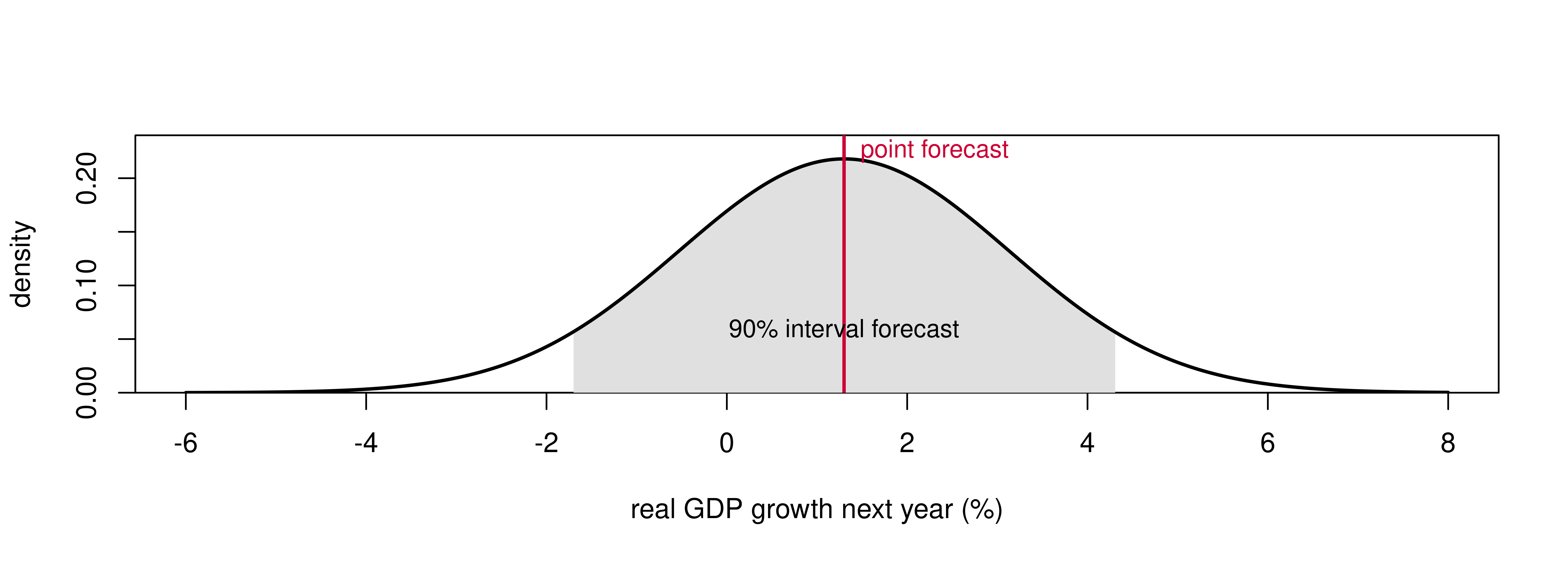
Point forecast. A single number. “Real GDP will grow 1.3% next year.” Usually the mean (or median) of the forecast distribution.
Interval forecast. A range with an attached probability. “With probability 90%, growth will be between -1.7\% and 4.3\%” — that is 1.3\% give or take three points. Its width is the message: it reports how much you do not know.
Density forecast. The whole distribution. “Growth is normal with mean 1.3% and standard deviation 1.83%.”
They nest
One density forecast for US real GDP growth, with the point and interval forecasts it contains:
The information ordering
\text{density} \;\succ\; \text{interval} \;\succ\; \text{point}
- From a density you can read off an interval at any confidence level, and a point forecast as its mean or median.
- From an interval you can take the midpoint as a point forecast.
- From a point forecast you can recover nothing about uncertainty.
So density forecasts must be the standard practice. Right?
In practice the ordering is reversed
Point forecasts are overwhelmingly the most common, intervals a distant second, densities rare. Two reasons:
- Cost of assumptions. A point forecast needs a conditional mean. An interval needs the whole error distribution — either an extra distributional assumption that may be wrong, or heavy simulation.
- Cost of processing. Point forecasts are easier to understand and act on. Extra information is not an advantage when the recipient cannot use it.
The most visible exception is the Bank of England’s fan chart, which has published density forecasts of inflation since 1996 and did a great deal to normalize the practice.
Probability forecasts
For event outcome and event timing objects, the natural statement is a probability.
- “The economy will be in recession in six months” is the analogue of a point forecast.
- “There is a 35% chance of recession within six months” is the analogue of a density forecast.
The second is strictly more useful, and it is what the New York Fed, the SPF, and every credit-risk model actually report.
Scoring probability forecasts needs its own loss function (the Brier score, the log score). Same principle as before: state the loss, then optimize against it.
4. The forecast horizon
What a step means
The forecast horizon h is the number of periods between now and the date being forecast. A step is one observation interval:
| Data frequency | One step | h = 12 |
|---|---|---|
| Annual | 1 year | 12 years |
| Quarterly | 3 months | 3 years |
| Monthly | 1 month | 1 year |
| Daily | 1 day | about 2 weeks |
So “a twelve-step-ahead forecast” is meaningless until you say what the data are.
Two conventions
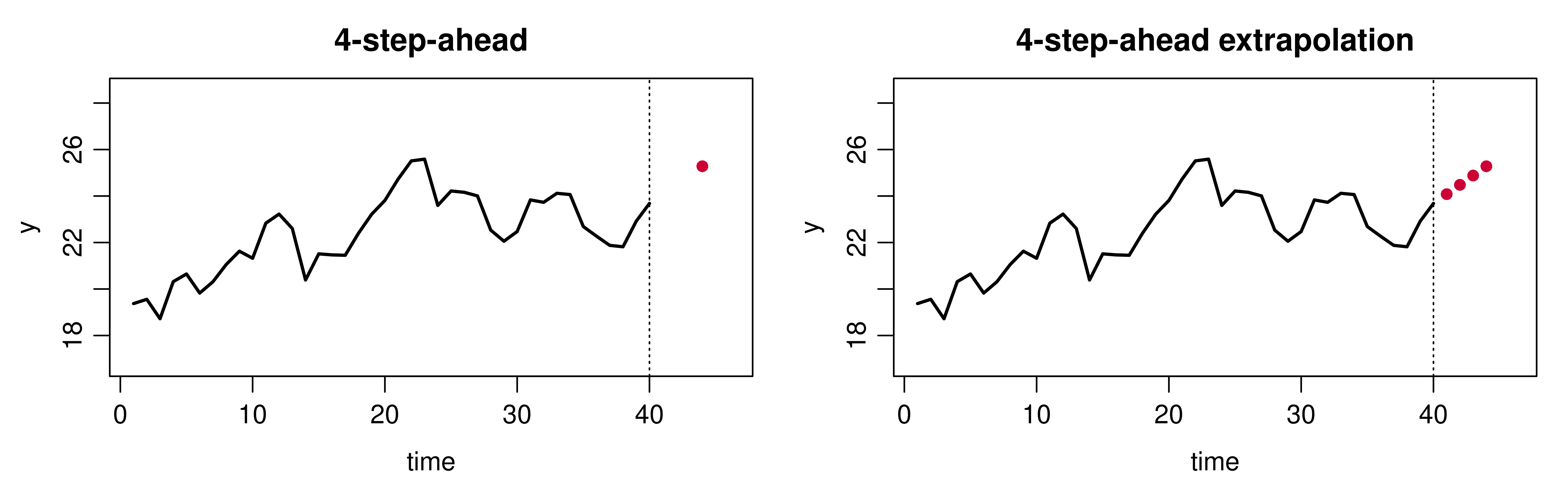
h-step-ahead forecast.
The horizon is fixed at h. Every month you produce a forecast for four months out, and only that one.
Used when one specific lead time drives a decision.
h-step-ahead extrapolation forecast.
The whole path \hat Y_{T+1\mid T}, \ldots, \hat Y_{T+h\mid T}.
Used for budgeting and planning, where you need the trajectory, not a single date.
Uncertainty grows with the horizon
How badly? Ask the data. For the simplest possible forecast — “no change from today” — the h-step error is just the h-period change.
##                 h=1  h=3  h=6 h=12 h=24  h=36  h=60
## error sd (%)    0.8 1.77 2.88 4.65 6.93  8.30 10.37
## relative to h=1 1.0 2.21 3.60 5.81 8.66 10.37 12.96
## sqrt(h)         1.0 1.73 2.45 3.46 4.90  6.00  7.75
Uncertainty grows with h at every horizon, and grows faster than \sqrt{h} — the rate you would see if monthly growth were unforecastable noise. That excess is direct evidence of persistence in industrial production growth. It stops widening beyond about two years, as the level begins to mean-revert.
The best model changes with the horizon
Every model is an approximation to the underlying dynamics. There is no reason the best approximation for one purpose should be best for another.
- At h=1, fine short-run dynamics dominate; an autoregression earns its keep.
- At h=60, the short-run dynamics have died out and what matters is the trend and the mean. A simple model usually wins.
Choose the model for the horizon you actually need.
This is why the model-selection criteria of Chapter 5 should, strictly, be applied at the horizon of interest — a point we return to when we discuss direct versus iterated multi-step forecasting.
5. The information set
What is in \Omega_T?
Univariate information set — the history of the series itself:
\Omega_T^{\text{uni}} = \{\, y_T,\, y_{T-1},\, \ldots,\, y_1 \,\}
Multivariate information set — other series too:
\Omega_T^{\text{multi}} = \{\, y_T, \ldots, y_1,\; x_T, \ldots, x_1 \,\}
Any forecast is conditional on the information used to make it, whether or not you say so. Being explicit about \Omega_T is what makes a forecast reproducible and evaluable.
Three model types
Explanatory model. Predictors do the work. \text{Demand}_{T+1} = f(\text{temperature},\, \text{income},\, \text{price},\, \ldots) + \varepsilon
Time series model. Only the past of the series itself. \text{Demand}_{T+1} = f(\text{Demand}_T,\, \text{Demand}_{T-1}, \ldots) + \varepsilon
Dynamic regression. Both. \text{Demand}_{T+1} = f(\text{Demand}_T, \ldots,\, \text{temperature}_{T+1}, \ldots) + \varepsilon
Why forecast with a pure time series model?
It looks like throwing information away. Four reasons it often wins:
- The system may not be understood. No credible structural model exists for many series worth forecasting.
- You would have to forecast the predictors first. To use temperature next month you need a forecast of temperature next month — errors compound.
- You may not care why. Prediction, not explanation, is the goal here (recall Lecture 3: confounding is not a problem for forecasting).
- It may simply be more accurate. Repeatedly demonstrated in forecasting competitions.
Information in real time
The information set is defined by what was available at T, not by what is in today’s spreadsheet.
- Publication lags. Q1 GDP is not published in Q1.
- Revisions. The first estimate of GDP growth differs, sometimes a lot, from the number in the file five years later.
- Ragged edges. Different series arrive on different days, so at any moment some are one month stale and others two.
A backtest run on final revised data can flatter a model badly.
Doing this properly requires real-time vintage data. For US macro series the Philadelphia Fed maintains one.
The information set in evaluation
When a forecast disappoints, there are two distinct questions:
- Could it be improved by using the same information more efficiently? (Is there signal left in the forecast errors?)
- Could it be improved by using more information? (Would adding a series help?)
The first is a testable property of the errors and is the basis of forecast evaluation later in the course. The second is a modelling decision — and is where the parsimony principle bites.
6. Methods and complexity
A complex world does not require a complex model
The phenomena we forecast are enormously complicated. It is tempting to conclude that our models should be too.
Decades of professional experience say the opposite.
Parsimony principle. Other things equal, simple models are preferable to complex models.
Why simple models win
- Estimation precision. Fewer parameters, estimated from the same data, are estimated better.
- Scrutiny. A small model can be understood, so anomalous behaviour gets spotted. A 200-parameter model that has quietly broken looks exactly like one that has not.
- Communication. Forecasts are used by people who must trust them. You can explain a small model.
- Less scope for data mining. Tailoring a model to maximize historical fit produces models that fit the past beautifully by construction and forecast the future miserably.
The cost of a parameter
Take a correctly specified regression with k estimated coefficients (the intercept included) and n observations. The expected squared error of a new observation is approximately
E\big[(Y_{\text{new}} - \hat Y_{\text{new}})^2\big] \;\approx\; \sigma^2\Big(1 + \tfrac{k}{n}\Big)
The \sigma^2 is irreducible; the \sigma^2 k / n is the price of having estimated the coefficients rather than known them.
Every extra parameter costs about \sigma^2/n out of sample, whether or not it helps.
A useless parameter pays nothing back. A marginally useful one may not pay for itself either.
Checking that claim
True process: an AR(1). We fit AR(p) for p = 1, \ldots, 12 on n = 60 observations, then score one genuinely new observation. Lags 2, \ldots, p are truly irrelevant, so any deterioration is pure variance.
set.seed(4354)
phi <- 0.6; n <- 60; pmax <- 12
one_draw <- function() {
  y <- as.numeric(arima.sim(list(ar = phi), n + pmax + 1, sd = 1))
  L <- embed(y, pmax + 1); tr <- seq_len(n); te <- n + 1
  sapply(1:pmax, function(p) {
    Z <- cbind(1, L[, seq_len(p) + 1, drop = FALSE])
    b <- qr.solve(Z[tr, , drop = FALSE], L[tr, 1])
    (L[te, 1] - sum(Z[te, ] * b))^2
  })
}
mc  <- rowMeans(replicate(4000, one_draw()))
tab <- rbind(simulated = mc, `sigma2(1 + k/n)` = 1 + (1:pmax + 1) / n)
round(`colnames<-`(tab, paste0("p=", 1:pmax))[, c(1, 2, 4, 6, 8, 10, 12)], 3)
## p=1 p=2 p=4 p=6 p=8 p=10 p=12
## simulated 1.048 1.065 1.109 1.154 1.189 1.251 1.292
## sigma2(1 + k/n) 1.033 1.050 1.083 1.117 1.150 1.183 1.217Checking that claim (cont.)
plot(1:pmax, mc, type = "b", pch = 16, lwd = 2, col = "#cc0035",
     ylim = range(mc, 1 + (1:pmax + 1)/n), xlab = "lags included, p",
     ylab = "out-of-sample MSE")
lines(1:pmax, 1 + (1:pmax + 1)/n, lwd = 2, lty = 2, col = "#354ca1")
legend("topleft", c("simulated", "sigma^2 (1 + k/n)"),
       col = c("#cc0035", "#354ca1"), lwd = 2, lty = c(1, 2), pch = c(16, NA), bty = "n")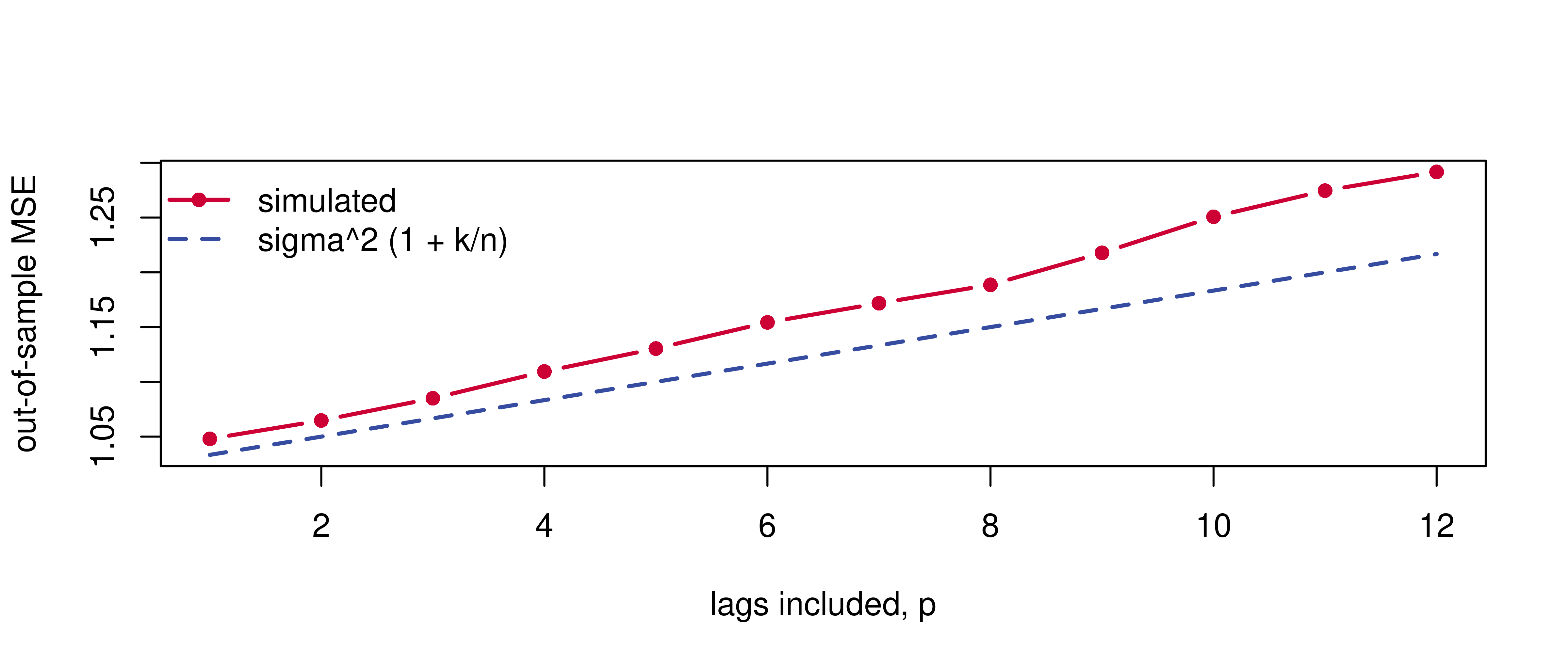
The formula tracks the slope. It sits a little low because the regressors here are lagged dependent variables, not fixed — the true cost of a parameter is worse than the textbook approximation.
The same picture on real data
Forecast monthly US industrial production growth with an AR(p). Estimate on the 1990s; score one-step-ahead forecasts over 2000–2019.
pmax  <- 24
L     <- embed(ip$growth[-1], pmax + 1)      # col 1 = y_t, col j+1 = y_{t-j}
dates <- ip$date[-(1:(pmax + 1))]
train <- dates >= as.Date("1990-01-01") & dates <= as.Date("1999-12-01")
test  <- dates >= as.Date("2000-01-01")

mse <- t(sapply(0:pmax, function(p) {
  Z <- cbind(1, L[, seq_len(p) + 1, drop = FALSE])
  b <- qr.solve(Z[train, , drop = FALSE], L[train, 1])
  c(in_sample  = mean((L[train, 1] - Z[train, , drop = FALSE] %*% b)^2),
    out_sample = mean((L[test,  1] - Z[test,  , drop = FALSE] %*% b)^2))
}))
rownames(mse) <- paste0("p=", 0:pmax)
t(round(mse[c(1, 3, 4, 5, 7, 13, 25), ], 3))
## p=0 p=2 p=3 p=4 p=6 p=12 p=24
## in_sample 0.265 0.258 0.247 0.247 0.245 0.229 0.207
## out_sample 0.507 0.442 0.401 0.410 0.415 0.418 0.458The same picture on real data (cont.)
matplot(0:pmax, mse, type = "b", pch = 16, lty = 1, lwd = 2,
        col = c("#354ca1", "#cc0035"), xlab = "lags included, p",
        ylab = "mean squared forecast error")
abline(v = which.min(mse[, 2]) - 1, lty = 3)
legend("left", c("in-sample (1990s)", "out-of-sample (2000-2019)"),
       col = c("#354ca1", "#cc0035"), pch = 16, lwd = 2, bty = "n")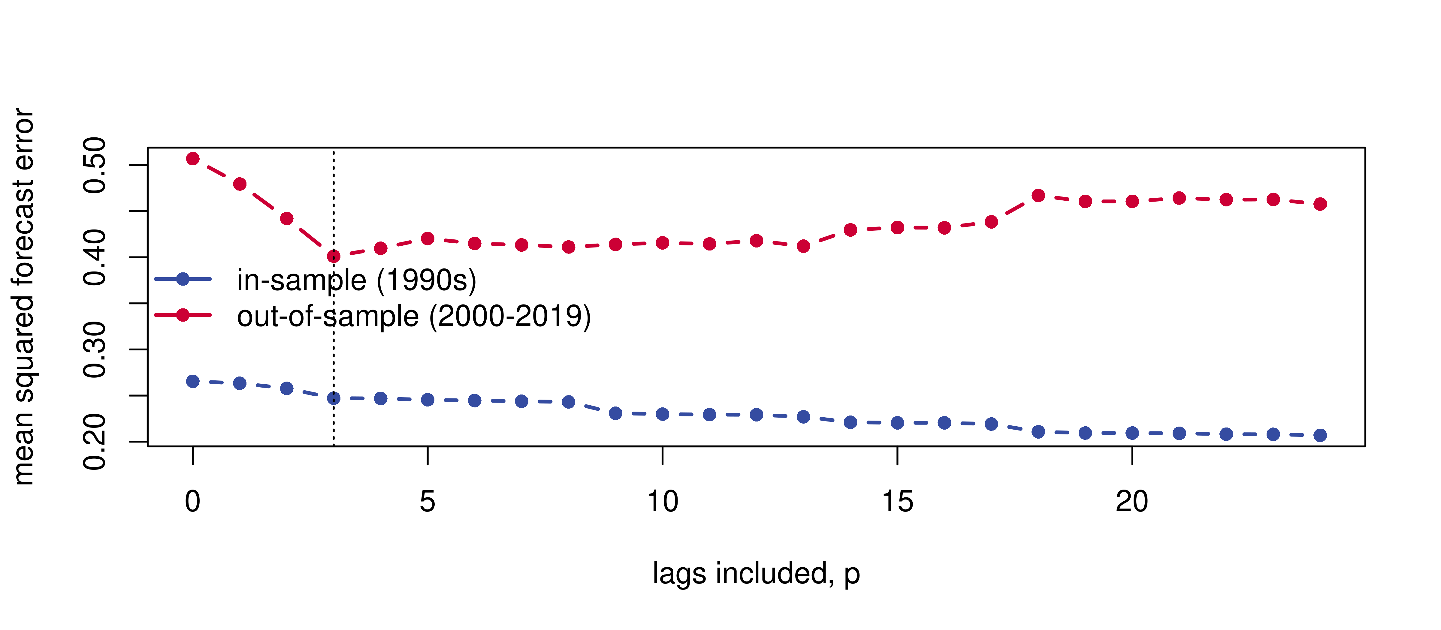
In-sample error falls with every lag added. Out-of-sample error bottoms out at p = 3 and is 14% worse by p = 24.
Data mining
The failure mode has a name. You try many specifications, keep the one that fits best, and report it as though it were the only one you tried.
- The reported R^2, t-statistics and p-values are then all wrong — they assume a single, pre-specified model.
- What you have fitted is partly the idiosyncrasies of this sample, which have no counterpart in the future.
Fit is not evidence of forecasting ability. Only out-of-sample performance is.
This is why the discipline of holding out data, or of a genuine pseudo-out-of-sample exercise, is not optional. Chapter 5 formalizes it with information criteria; Chapter 12 with forecast evaluation.
The shrinkage principle
Related to parsimony but distinct:
Shrinkage principle. Imposing restrictions on forecasting models often improves forecast performance.
The name comes from coaxing — “shrinking” — forecasts toward something simple: toward zero, toward the sample mean, toward another model’s forecast.
Parsimony is a special case: setting a coefficient to zero is the most brutal possible restriction.
Shrinkage, seen
Take the over-parameterized AR(12) from the simulation and shrink its forecast toward the sample mean:
\hat Y^{(\lambda)} \;=\; \lambda \,\hat Y_{\text{AR}(12)} \;+\; (1-\lambda)\,\bar y
set.seed(4354)
lam <- seq(0, 1, by = 0.1)
one_shrink <- function(phi = 0.6, n = 60, p = 12) {
  y  <- as.numeric(arima.sim(list(ar = phi), n + p + 1, sd = 1))
  L  <- embed(y, p + 1); Z <- cbind(1, L[, -1]); tr <- seq_len(n)
  b  <- qr.solve(Z[tr, ], L[tr, 1])
  (L[n + 1, 1] - (lam * sum(Z[n + 1, ] * b) + (1 - lam) * mean(L[tr, 1])))^2
}
round(setNames(rowMeans(replicate(4000, one_shrink())), lam), 3)
## 0 0.1 0.2 0.3 0.4 0.5 0.6 0.7 0.8 0.9 1
## 1.667 1.558 1.466 1.389 1.328 1.283 1.253 1.239 1.241 1.258 1.292\lambda = 1 is the unrestricted model; \lambda = 0 ignores the data entirely. The best forecast is neither.
Why shrinkage works
It is the bias–variance decomposition again, from Lecture 3:
E\big[(Y - \hat Y)^2\big] = \sigma^2 + \underbrace{\big(E\hat Y - E(Y\mid \Omega)\big)^2}_{\text{bias}^2} + \underbrace{\operatorname{Var}(\hat Y)}_{\text{variance}}
Shrinking toward a constant introduces bias. It also cuts variance, because a constant has none. For small \lambda away from 1, the variance saving is first-order and the bias cost is second-order.
Gauss–Markov told us OLS is best among unbiased estimators. For forecasting, unbiasedness is not worth what it costs.
Ridge, lasso, Bayesian priors, forecast combination, and the shrunken covariance matrices used in portfolio choice are all this idea. We meet several of them later.
Simple, not naive
KISS: Keep It Sophisticatedly Simple.
Parsimony is not an excuse for laziness. A parsimonious model is one that has been thought about until only the parts that earn their keep remain.
- Fitting a straight line to a series with obvious seasonality is naive, not simple.
- Fitting a 200-parameter model because the software allowed it is complex, not sophisticated.
The skill is knowing which complications matter. That is what the rest of the course teaches.
References
Additional resources
- Textbooks
- Diebold, F.X. Elements of Forecasting, 4th edition, Chapter 3 — the six considerations.
- Hyndman, R.J. and Athanasopoulos, G. Forecasting: Principles and Practice (3rd ed.), Chapter 1 — freely available online.
- Elliott, G. and Timmermann, A. Economic Forecasting (2016), Chapters 2–3 — the graduate treatment of loss functions and optimal forecasts.
- On loss functions and optimal prediction
- Granger, C.W.J. (1969), “Prediction with a Generalized Cost of Error Function,” Operational Research Quarterly, 20, 199–207.
- Christoffersen, P.F. and Diebold, F.X. (1997), “Optimal Prediction Under Asymmetric Loss,” Econometric Theory, 13, 808–817.
- Data
data/2024-07-fredmd.csv— FRED-MD, the monthly US macro panel (McCracken and Ng, 2016). Vintage July 2024.- Real-time vintages: the Philadelphia Fed’s Real-Time Data Research Center.