library(AER)
data("CPS1985")
cps <- CPS1985
cps$lwage <- log(cps$wage)   # log hourly wage, used from here on
dim(cps)
## [1] 534 12Review Session: The Linear Regression Model
08 September 2026
A forecast is a conditional expectation: given what I observe today, what is my best guess of tomorrow?
The linear regression model is the workhorse for computing that guess.
So we spend one session making sure the machinery is solid: what OLS is, when it is good, and what its standard errors mean.
Throughout the session we use one dataset: a random sample of 534 workers from the May 1985 Current Population Survey, shipped with the AER package.
## [1] 534 12## 'data.frame': 534 obs. of 12 variables:
## $ wage : num 5.1 4.95 6.67 4 7.5 ...
## $ education : num 8 9 12 12 12 13 10 12 16 12 ...
## $ experience: num 21 42 1 4 17 9 27 9 11 9 ...
## $ age : num 35 57 19 22 35 28 43 27 33 27 ...
## $ ethnicity : Factor w/ 3 levels "cauc","hispanic",..: 2 1 1 1 1 1 1 1 1 1 ...
## $ region : Factor w/ 2 levels "south","other": 2 2 2 2 2 2 1 2 2 2 ...
## $ gender : Factor w/ 2 levels "male","female": 2 2 1 1 1 1 1 1 1 1 ...
## $ occupation: Factor w/ 6 levels "worker","technical",..: 1 1 1 1 1 1 1 1 1 1 ...
## $ sector : Factor w/ 3 levels "manufacturing",..: 1 1 1 3 3 3 3 3 1 3 ...
## $ union : Factor w/ 2 levels "no","yes": 1 1 1 1 1 2 1 1 1 1 ...
## $ married : Factor w/ 2 levels "no","yes": 2 2 1 1 2 1 1 1 2 1 ...
## $ lwage : num 1.63 1.6 1.9 1.39 2.01 ...\text{wage}_i \;=\; f(\text{education}_i, \text{experience}_i, \ldots) \;+\; U_i
Three things we might mean by it:
Same equation, same estimates, three different questions. We come back to this.
A random variable X has a distribution. Two summaries do most of the work.
Expectation — the center
E(X) = \sum_x x \cdot f(x)
Linear: E(aX + bY + c) = aE(X) + bE(Y) + c.
Variance — the spread
\mathrm{Var}(X) = E\big[(X - E X)^2\big] = E(X^2) - (EX)^2
Not linear: \mathrm{Var}(aX + b) = a^2 \mathrm{Var}(X).
Covariance measures co-movement; correlation makes it unit-free.
\mathrm{Cov}(X,Y) = E\big[(X - EX)(Y - EY)\big], \qquad \rho_{XY} = \frac{\mathrm{Cov}(X,Y)}{\sqrt{\mathrm{Var}(X)\mathrm{Var}(Y)}} \in [-1, 1]
X and Y move together. Three stories, all consistent with the same \rho:
Case 3 is the reason a regression coefficient is not automatically a causal effect. It will return as omitted variable bias.
For forecasting, cases 1–3 are all fine! We only need X to predict Y, not to move it.
The object at the heart of everything: E(Y \mid X = x) — the average of Y among units whose X equals x.
When X is discrete, this is just a group mean:
The difference in log wages between union and non-union members is 0.286 — roughly a 29% union premium, before controlling for anything.
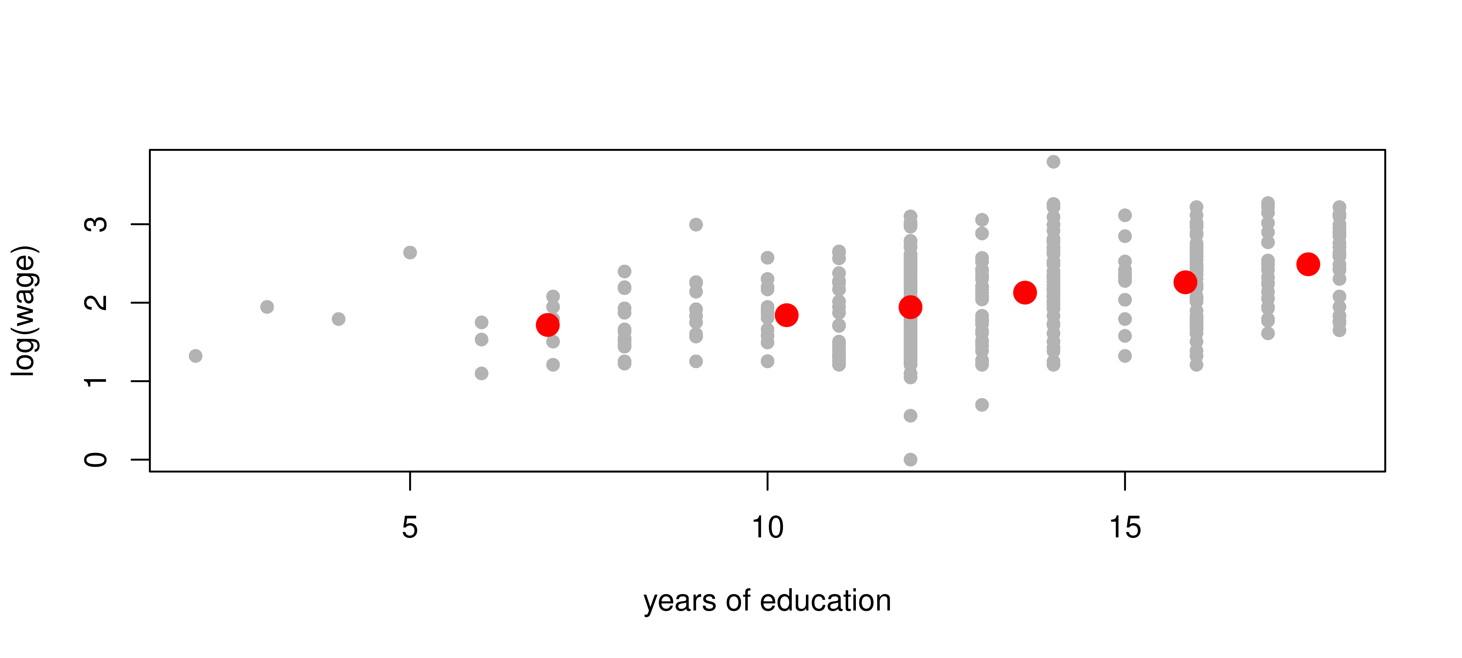
With continuous X we cannot condition on each value — cells are empty. So we bin, or we impose a functional form.
bins   <- cut(cps$education, breaks = c(0, 8, 11, 12, 14, 16, 18))
cell_y <- tapply(cps$lwage,     bins, mean)   # average log wage in the bin
cell_x <- tapply(cps$education, bins, mean)   # average education in the bin
plot(cps$education, cps$lwage, pch = 16, col = "grey70",
     xlab = "years of education", ylab = "log(wage)")
points(cell_x, cell_y, pch = 19, col = "red", cex = 1.6)Law of iterated expectations
E\big[\,E(Y \mid X)\,\big] = E(Y)
The average of the group averages (weighted by group size) is the overall average.
Conditioning theorem
E\big[\,g(X)\,Y \mid X\,\big] = g(X)\, E(Y \mid X)
Once you condition on X, any function of X is a constant.
Together these two lines drive every unbiasedness proof in the course.
Assume the conditional expectation is linear:
E(Y \mid X) = \beta_0 + \beta_1 X
Then, mechanically,
\beta_1 = \frac{\mathrm{Cov}(X,Y)}{\mathrm{Var}(X)}, \qquad \beta_0 = E(Y) - \beta_1 E(X)
Now suppose a structural model generates the data:
Y = \beta_0 + \beta_1 X + U, \qquad U = \text{everything else that matters}
\beta_1 is the effect of moving X by one unit, holding U fixed.
This is only recoverable from data if
E(U \mid X) = 0
i.e. the unobservables are mean-independent of X. That is an assumption about the world, not something the data can confirm.
Ability is in U and is surely correlated with education \Rightarrow the wage regression is not causal.
We observe X = x^* and want to guess the associated Y^*.
Choose the forecast \hat{Y}^* to minimize expected squared error. The solution is
\hat{Y}^* = E(Y \mid X = x^*)
Whatever the question, the sample answer is the same: choose the line that fits best in squared error.
(\hat\beta_0, \hat\beta_1) = \arg\min_{b_0, b_1} \sum_{i=1}^n (Y_i - b_0 - b_1 X_i)^2
| Reading | What \beta_1 means | What must be true |
|---|---|---|
| Descriptive | slope of the CEF | E(Y\mid X) is linear |
| Causal | ceteris paribus effect | E(U \mid X) = 0 |
| Forecast | best linear guess | x^* is in the support of X |
Minimize g(b_0, b_1) = \sum_i (Y_i - b_0 - b_1 X_i)^2. First order conditions:
\frac{\partial g}{\partial b_0} = 0 \;\Rightarrow\; -2\sum_i (Y_i - \hat\beta_0 - \hat\beta_1 X_i) = 0 \frac{\partial g}{\partial b_1} = 0 \;\Rightarrow\; -2\sum_i (Y_i - \hat\beta_0 - \hat\beta_1 X_i)X_i = 0
Solving gives the sample analog of the population formula:
\hat\beta_1 = \frac{\sum_i (X_i - \bar X)(Y_i - \bar Y)}{\sum_i (X_i - \bar X)^2} = \frac{\widehat{\mathrm{Cov}}(X,Y)}{\widehat{\mathrm{Var}}(X)}, \qquad \hat\beta_0 = \bar Y - \hat\beta_1 \bar X
lm()## intercept slope
## 1.05988987 0.07675856Identical, as they must be. From here on we let lm() do the arithmetic.
lm output##
## Call:
## lm(formula = lwage ~ education, data = cps)
##
## Residuals:
## Min 1Q Median 3Q Max
## -1.98099 -0.37155 0.03391 0.34975 1.66098
##
## Coefficients:
## Estimate Std. Error t value Pr(>|t|)
## (Intercept) 1.059890 0.107432 9.866 <2e-16 ***
## education 0.076759 0.008091 9.487 <2e-16 ***
## ---
## Signif. codes: 0 '***' 0.001 '**' 0.01 '*' 0.05 '.' 0.1 ' ' 1
##
## Residual standard error: 0.4885 on 532 degrees of freedom
## Multiple R-squared: 0.1447, Adjusted R-squared: 0.1431
## F-statistic: 90.01 on 1 and 532 DF, p-value: < 2.2e-16\hat Y_i = \hat\beta_0 + \hat\beta_1 X_i \quad\text{(fitted value)}, \qquad \hat U_i = Y_i - \hat Y_i \quad\text{(residual)}
The residual \hat U_i is not the error U_i.
These are the two first order conditions, rewritten. They hold in every OLS regression, no assumptions required.
## [1] 8.014206e-15## [1] 3.089543e-14Consequences worth remembering:
Because \hat U is orthogonal to \hat Y, total variation splits cleanly:
\underbrace{\sum_i (Y_i - \bar Y)^2}_{SST} = \underbrace{\sum_i (\hat Y_i - \bar Y)^2}_{SSE \;(\text{explained})} + \underbrace{\sum_i \hat U_i^2}_{SSR \;(\text{residual})}
R^2 \equiv \frac{SSE}{SST} = 1 - \frac{SSR}{SST} \in [0, 1]
The share of the variation in Y that the regression accounts for.
R^2 = 0.145. Education explains 14% of the variation in log wages. Is that bad?
Linearity is a restriction on the parameters, not on the variables. We are free to transform Y and X.
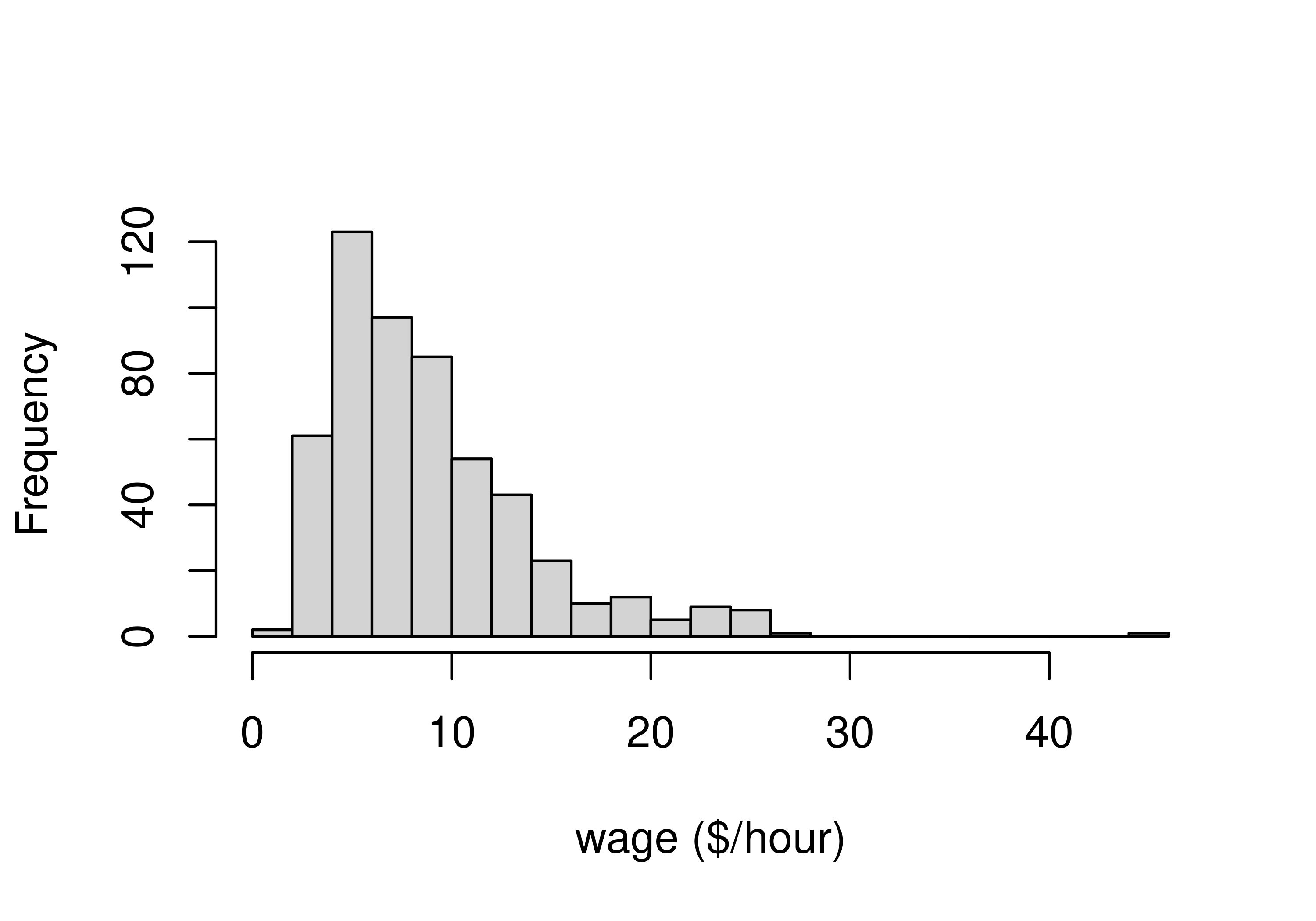
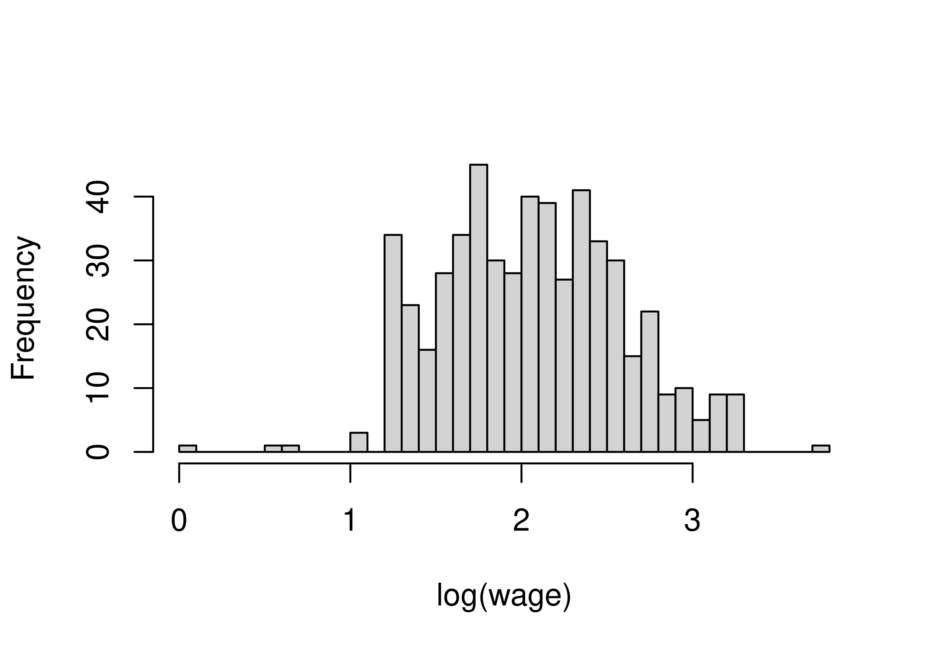
Logs tame the right skew, and they buy us an interpretation.
| Model | Equation | Interpretation of \beta_1 |
|---|---|---|
| level–level | Y = \beta_0 + \beta_1 X | \Delta Y = \beta_1 \Delta X |
| log–level | \log Y = \beta_0 + \beta_1 X | \%\Delta Y \approx 100\,\beta_1\, \Delta X |
| level–log | Y = \beta_0 + \beta_1 \log X | \Delta Y \approx (\beta_1/100)\, \%\Delta X |
| log–log | \log Y = \beta_0 + \beta_1 \log X | elasticity: \%\Delta Y \approx \beta_1 \%\Delta X |
Rescaling a variable rescales its coefficient, and nothing else. Multiply Y by c: every coefficient is multiplied by c. Multiply X_j by c: \hat\beta_j is divided by c.
##          (Intercept)  education
## baseline  -0.7459797  0.7504608
## Y_x_100  -74.5979668 75.0460751
## X_x_12    -0.7459797  0.0625384
Row 2: both coefficients multiplied by 100. Row 3: the slope divided by 12, intercept untouched.
R^2 and every t-statistic are unchanged: units are not information.
##          baseline   Y_x_100    X_x_12
## R2      0.1458645 0.1458645 0.1458645
## t_slope 9.5316300 9.5316300 9.5316300
Note that taking logs is not a rescaling. \log(cY) = \log c + \log Y shifts the intercept only, leaving the slope alone.
\hat\beta_1 is computed from a sample. Draw a different sample, get a different number.
So \hat\beta_1 has a sampling distribution, and we judge estimators by its features:
Bias — is it centered on the truth?
\mathrm{Bias}(\hat\beta_1) = E(\hat\beta_1) - \beta_1
Variance — how tightly?
\mathrm{Var}(\hat\beta_1) = E\big[(\hat\beta_1 - E\hat\beta_1)^2\big]
Neither alone is enough: \hat\beta_1 \equiv 7 has zero variance and is useless; a wildly noisy unbiased estimator is useless too.
SLR.1 (Linear in parameters). In the population, Y = \beta_0 + \beta_1 X + U.
SLR.2 (Random sampling). \{(X_i, Y_i)\}_{i=1}^n is an i.i.d. sample from that population.
SLR.3 (Sample variation in X). The X_i are not all equal. Otherwise the denominator of \hat\beta_1 is zero.
SLR.4 (Mean independence). E(U \mid X) = 0.
Under SLR.1–SLR.4, E(\hat\beta_0) = \beta_0 and E(\hat\beta_1) = \beta_1.
SLR.3 is checkable in the data. SLR.4 is never checkable — it is the whole ballgame in causal work.
Write \hat\beta_1 as truth plus noise:
\hat\beta_1 = \beta_1 + \frac{\sum_i (X_i - \bar X) U_i}{\sum_i (X_i - \bar X)^2}
Condition on all the X’s. The denominator is then a constant, and
E(\hat\beta_1 \mid \mathbf{X}) = \beta_1 + \frac{\sum_i (X_i - \bar X)\, E(U_i \mid \mathbf{X})}{\sum_i (X_i - \bar X)^2} = \beta_1
using SLR.4. Then apply the law of iterated expectations: E(\hat\beta_1) = E[E(\hat\beta_1 \mid \mathbf{X})] = \beta_1.
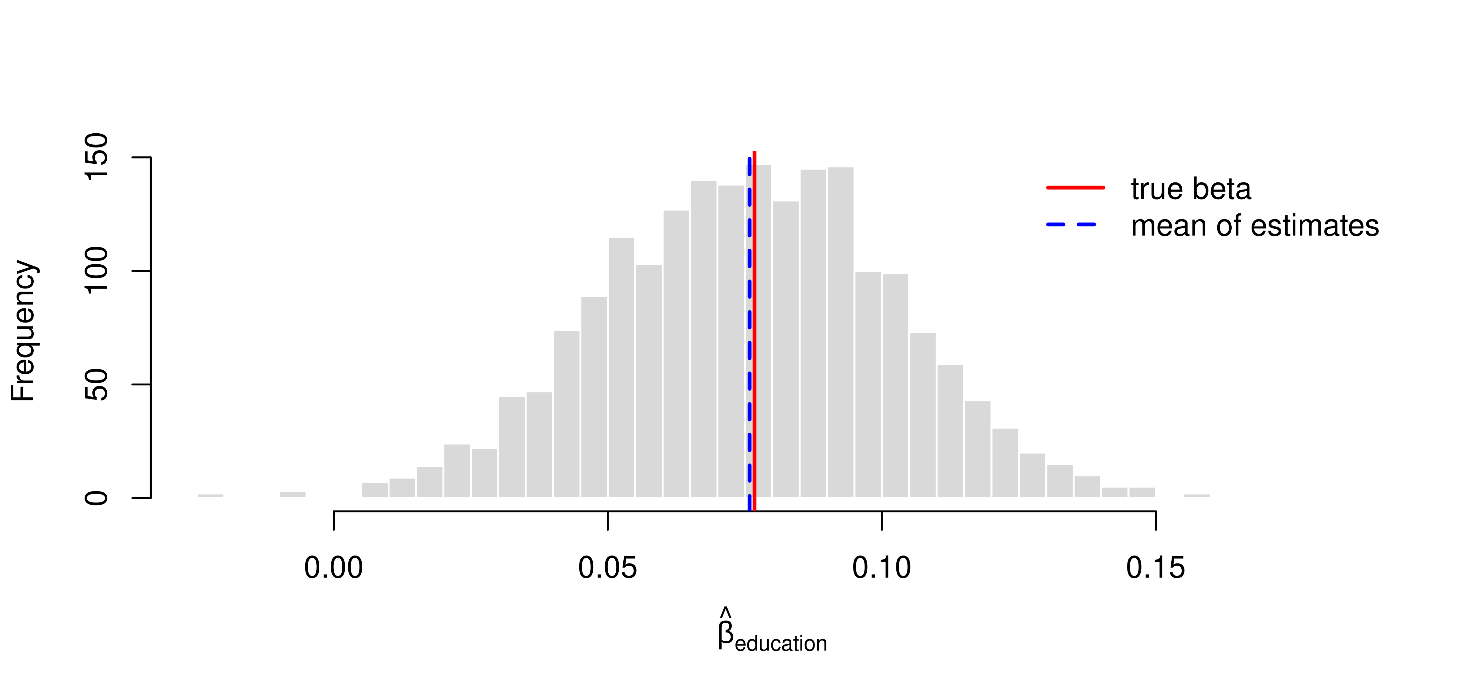
Treat the fitted simple regression as if it were the population, then draw 2000 samples of 50 workers each.
set.seed(4354)
pop  <- lm(lwage ~ education, data = cps)
beta <- coef(pop)          # the "true" (b0, b1) in this experiment
sig  <- summary(pop)$sigma # the "true" error sd
educ <- cps$education      # the population of X values to resample

draw_beta <- function(n) {
  i <- sample(length(educ), n, replace = TRUE)      # SLR.2: random sampling
  y <- beta[1] + beta[2] * educ[i] + rnorm(n, sd = sig)  # SLR.1 and SLR.4 hold
  coef(lm(y ~ educ[i]))[2]                          # keep the slope
}
b_hat <- replicate(2000, draw_beta(50))hist(b_hat, breaks = 40, col = "grey85", border = "white",
main = "", xlab = expression(hat(beta)[education]))
abline(v = beta[2], col = "red", lwd = 2)
abline(v = mean(b_hat), col = "blue", lwd = 2, lty = 2)
legend("topright", c("true beta", "mean of estimates"),
col = c("red", "blue"), lwd = 2, lty = c(1, 2), bty = "n")Any single estimate can be far off. The center is right.
One regressor is almost never enough. The wage equation needs experience, union status, and much else — and the reason is not just fit, it is bias.
The model becomes
Y = \beta_0 + \beta_1 X_1 + \beta_2 X_2 + \cdots + \beta_k X_k + U
and \beta_j is now the effect of X_j holding the other regressors fixed.
The four assumptions carry over almost unchanged, renamed MLR:
MLR.1 (Linear in parameters). The population model is the equation above.
MLR.2 (Random sampling). \{(X_{i1},\ldots,X_{ik}, Y_i)\}_{i=1}^n is i.i.d.
MLR.3 (No perfect collinearity). No regressor is constant, and no regressor is an exact linear combination of the others.
MLR.4 (Mean independence). E(U \mid X_1, \ldots, X_k) = 0.
Under MLR.1–MLR.4, E(\hat\beta_j) = \beta_j for every j.
SLR.3 only asked that X vary. With many regressors we also need them to vary independently of each other.
If X_2 = 2 X_1, then “hold X_1 fixed and move X_2” is not a question the data can answer — no such comparison exists in the sample.
Classic ways to break it:
education in years and education in months.age, education, and experience when experience = age - education - 6.That last one is not hypothetical in our data. We come back to it in the next section.
Suppose the truth is a “long” model, but we run a “short” one:
\text{long:} \quad Y = \beta_0 + \beta_1 X_1 + \beta_2 X_2 + U \text{short:} \quad Y = \tilde\beta_0 + \tilde\beta_1 X_1 + \varepsilon
Then, letting \tilde\delta_1 be the slope from regressing X_2 on X_1,
\boxed{\;\tilde\beta_1 = \hat\beta_1 + \hat\beta_2 \tilde\delta_1\;}
The bias is the product of two signs:
The boxed line is an algebraic identity between three regressions run on one sample — it holds exactly, always. The population statement E(\tilde\beta_1) - \beta_1 = \beta_2 \delta_1 is what makes it a statement about bias, and that one needs MLR.1–4 for the long model.
Omit experience from the wage equation:
##    short_slope.education long_plus_bias.education
## 0.07675856 0.07675856| sign | reading | |
|---|---|---|
| \hat\beta_2 (experience on wage) | + | experience raises wages |
| \tilde\delta_1 (education on experience) | - | the more school, the less time worked |
| bias | - | the short regression understates the return to schooling |
\text{Bias}(\tilde\beta_1) = \beta_2 \cdot \delta_1
| \mathrm{Corr}(X_1, X_2) > 0 | \mathrm{Corr}(X_1, X_2) < 0 | |
|---|---|---|
| \beta_2 > 0 | upward bias | downward bias |
| \beta_2 < 0 | downward bias | upward bias |
\delta_1 = \mathrm{Cov}(X_1,X_2)/\mathrm{Var}(X_1), so \delta_1 and \mathrm{Corr}(X_1,X_2) always share a sign. The table is easier to remember in terms of the correlation.
This table is how you argue about a paper you cannot re-estimate: “they omitted ability, ability raises wages, ability is positively correlated with schooling, so their estimate is too big.”
If \beta_2 = 0 or \delta_1 = 0, there is no bias. Omitting an irrelevant variable, or one uncorrelated with X_1, costs you nothing in bias.
The multiple regression coefficient has a two-step representation:
\hat\beta_1 = \frac{\sum_i \hat r_{i1} Y_i}{\sum_i \hat r_{i1}^2}
where \hat r_{i1} are the residuals from regressing X_1 on all other regressors.
\hat\beta_1 uses only the part of X_1 that is orthogonal to the other regressors.
This is the precise content of “holding the other variables constant”:
Keep the denominator in view. If X_1 is well explained by the other regressors, \hat r_{i1} is tiny, and dividing by \sum_i \hat r_{i1}^2 blows up the variance. That is the whole story of the next section.
MLR.5 (Homoskedasticity). The error variance does not depend on the regressors:
\mathrm{Var}(U \mid X_1, \ldots, X_k) = \sigma^2
Under MLR.1–MLR.5,
\mathrm{Var}(\hat\beta_j \mid \mathbf{X}) = \frac{\sigma^2}{SST_j\,(1 - R_j^2)}
where SST_j = \sum_i (X_{ij} - \bar X_j)^2 and R_j^2 is the R^2 from regressing X_j on all the other regressors.
Three levers, all intuitive:
fit3 <- lm(lwage ~ education + experience + union, data = cps)

sig2 <- sum(resid(fit3)^2) / fit3$df.residual         # sigma-hat squared
Rj2  <- summary(lm(education ~ experience + union,
                   data = cps))$r.squared             # R_j^2 for education
SSTj <- sum((cps$education - mean(cps$education))^2)

c(by_hand = sqrt(sig2 / (SSTj * (1 - Rj2))),
  from_lm = summary(fit3)$coefficients["education", "Std. Error"])
## by_hand from_lm
## 0.008130037 0.008130037The reported standard error is exactly \hat\sigma / \sqrt{SST_j (1 - R_j^2)}. Nothing mysterious.
In this dataset experience is defined as age - education - 6. So the three variables are nearly linearly dependent.
Exactly one of 534 workers breaks the identity.
##  education experience        age
## 229.5738 5147.9190 4611.4008lm() would drop a variable with an NA coefficient.Lesson: collinearity is a precision problem, not a bias problem. It is a statement about your data, not about your model being wrong.
Under MLR.1–MLR.5, the OLS estimators are BLUE:
Best Linear Unbiased Estimators.
Read the acronym carefully. OLS has the smallest variance among estimators that are
Note what is not required: normality of U plays no role here.
And note where it breaks: if MLR.5 fails (heteroskedasticity), OLS stays unbiased but is no longer best, and the usual standard errors are wrong.
Experience should raise wages at a decreasing rate. Add a square:
##     (Intercept)       education      experience I(experience^2)    genderfemale
##         0.58028         0.09074         0.03445        -0.00052        -0.23089
##        unionyes
##         0.20217
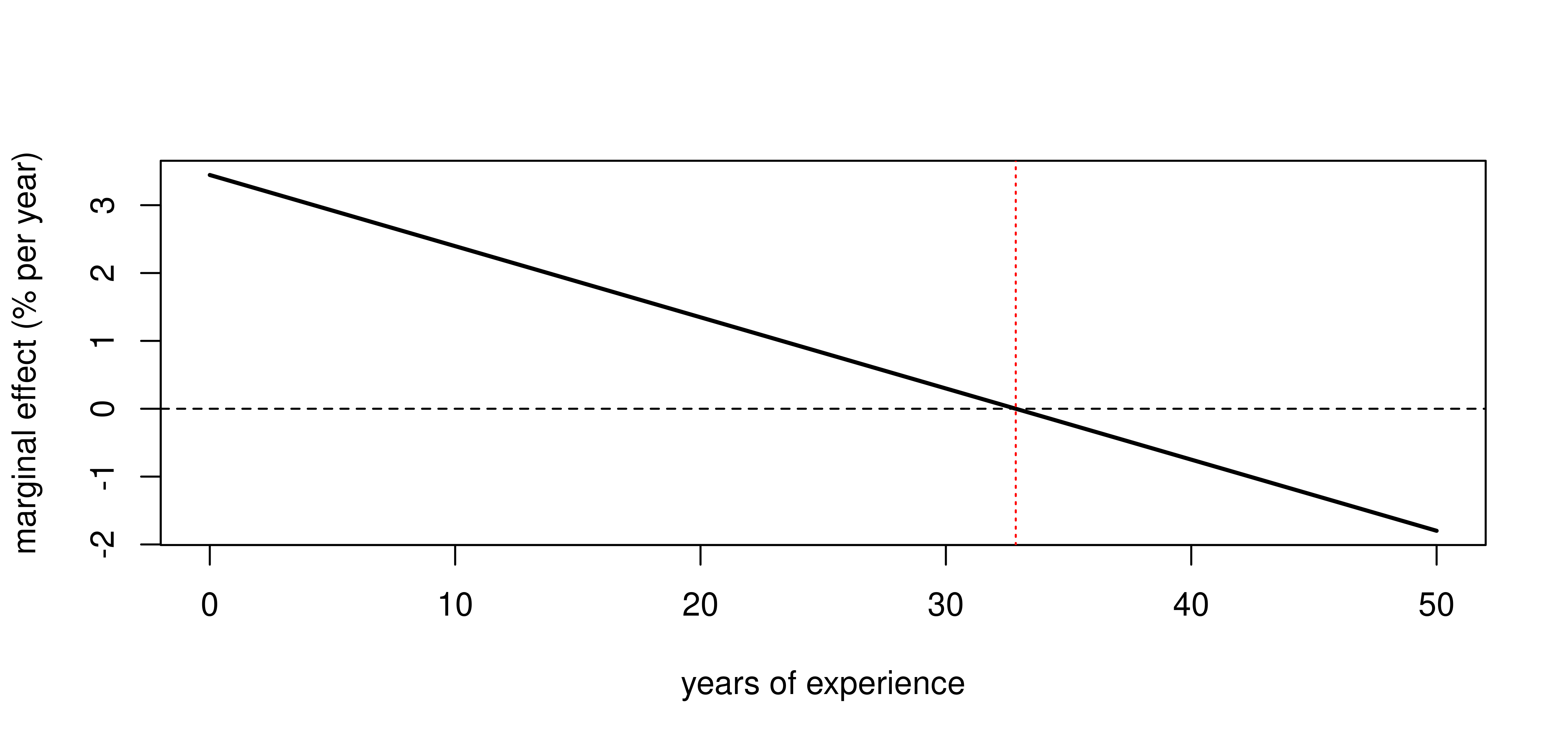
The marginal effect is now a function of experience:
\frac{\partial \widehat{\log(\text{wage})}}{\partial \text{exper}} = \hat\beta_2 + 2\hat\beta_3\,\text{exper}
Peak at \text{exper}^* = -\hat\beta_2 / (2\hat\beta_3) = 32.8 years.
Does the return to schooling differ for union members?
##                    Estimate Std. Error t value Pr(>|t|)
## education            0.0950     0.0085 11.1780   0.0000
## unionyes             0.5351     0.2504  2.1373   0.0330
## education:unionyes  -0.0257     0.0189 -1.3576   0.1752
\frac{\partial \widehat{\log(\text{wage})}}{\partial \text{educ}} = \hat\beta_{\text{educ}} + \hat\beta_{\text{educ}\times\text{union}} \cdot \mathbb{1}\{\text{union}\}
So the return is 9.5% for non-union workers and 6.9% for union members. But the interaction has p = 0.18: we cannot reject that the two are the same.
Two traps. education alone is the effect for non-union workers, not an average; and unionyes = 0.54 is the premium at zero years of schooling, an extrapolation far outside the data.
set.seed(4354)
sapply(list(
  "educ"                = lwage ~ education,
  "+ exper"             = lwage ~ education + experience,
  "+ exper^2"           = lwage ~ education + experience + I(experience^2),
  "+ gender, union"     = lwage ~ education + experience + I(experience^2) +
                                  gender + union,
  "+ pure noise"        = lwage ~ education + experience + I(experience^2) +
                                  gender + union + rnorm(nrow(cps))
), function(f) round(summary(lm(f, data = cps))$r.squared, 4))
## educ + exper + exper^2 + gender, union + pure noise
## 0.1447 0.2115 0.2382 0.3175 0.3194Even a column of random numbers raises R^2. Adding a regressor can never increase SSR, because the old coefficients remain available with the new one set to zero.
Penalize for the degrees of freedom spent:
\bar R^2 = 1 - \frac{SSR/(n-k-1)}{SST/(n-1)} = 1 - (1 - R^2)\frac{n-1}{n-k-1}
Add 40, then 120, columns of pure noise to the wage equation:
set.seed(4354)
NZ  <- matrix(rnorm(nrow(cps) * 120), nrow(cps))  # 120 junk regressors
f   <- lwage ~ education + experience + I(experience^2) + gender + union
fit <- function(m) c(k = m$rank - 1, R2 = summary(m)$r.squared,
                     adj_R2 = summary(m)$adj.r.squared)

round(cbind(none    = fit(lm(f, data = cps)),
            plus40  = fit(lm(update(f, . ~ . + NZ[, 1:40]),  data = cps)),
            plus120 = fit(lm(update(f, . ~ . + NZ[, 1:120]), data = cps))), 4)
## none plus40 plus120
## k 5.0000 45.0000 125.0000
## R2 0.3175 0.3671 0.4764
## adj_R2 0.3111 0.3087 0.3160R^2 climbs from 0.32 to 0.48 on nothing but noise. \bar R^2 does not move.
The penalty removes the mechanical drift: \bar R^2 is roughly an unbiased estimate of the population R^2, so adding junk leaves it where it was.
But “does not drift” is weaker than “picks the right model”. How often does \bar R^2 actually go down when we add 40 noise columns?
A coin flip: half the time \bar R^2 waves 40 worthless regressors through. The right instinct, the wrong tool — which is where we end.
To get exact small-sample distributions we add one more assumption.
MLR.6 (Normality). U \mid X_1, \ldots, X_k \sim \mathcal{N}(0, \sigma^2), independent of the regressors.
MLR.1–MLR.6 together are the classical linear model (CLM). Under it,
\hat\beta_j \sim \mathcal{N}\big(\beta_j,\; \mathrm{Var}(\hat\beta_j)\big) \quad\Longrightarrow\quad \frac{\hat\beta_j - \beta_j}{\mathrm{sd}(\hat\beta_j)} \sim \mathcal{N}(0,1)
But \sigma is unknown. Replacing it with \hat\sigma costs us the normal and buys a t:
T = \frac{\hat\beta_j - \beta_j}{\mathrm{se}(\hat\beta_j)} \sim t_{\,n-k-1}
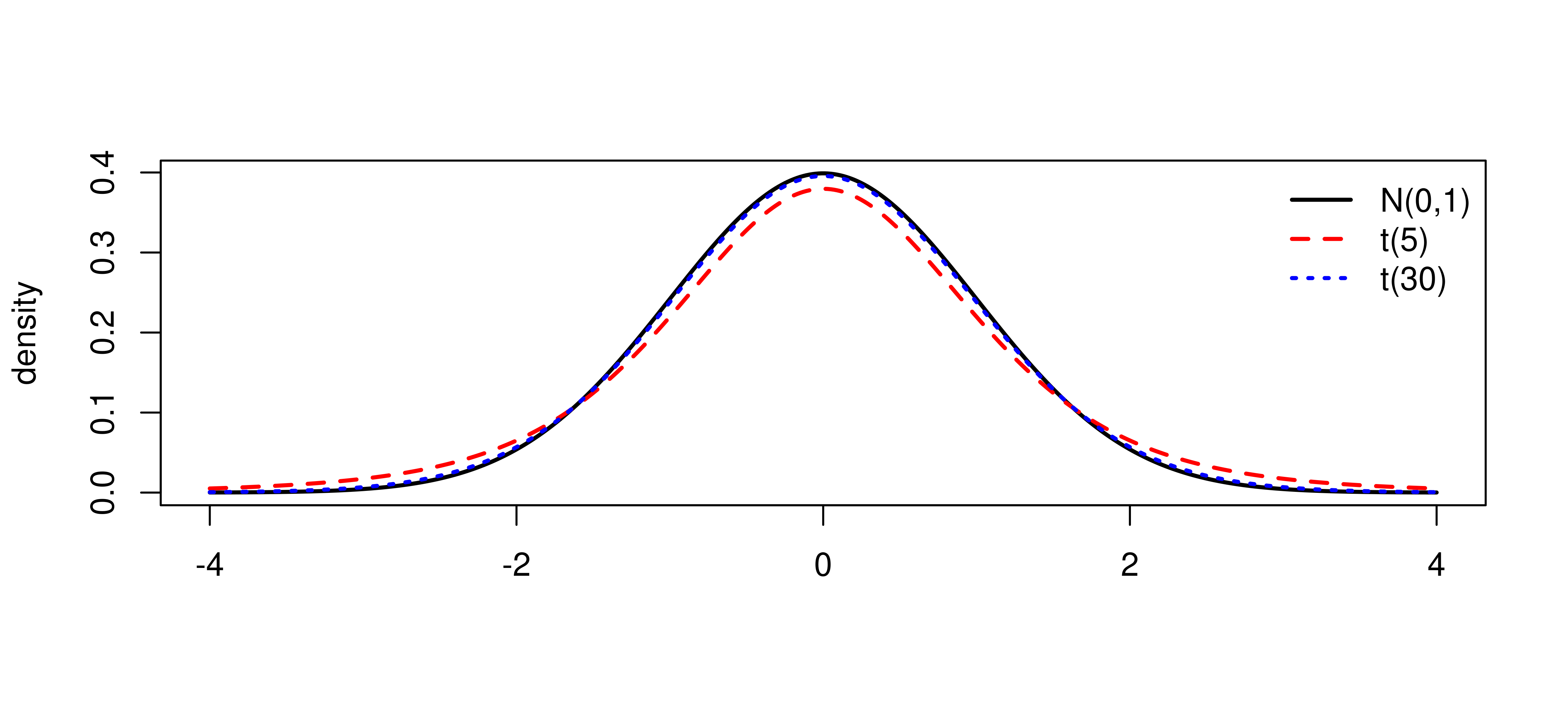
x <- seq(-4, 4, length.out = 400)
plot(x, dnorm(x), type = "l", lwd = 2, xlab = "", ylab = "density")
lines(x, dt(x, df = 5),  col = "red",  lwd = 2, lty = 2)
lines(x, dt(x, df = 30), col = "blue", lwd = 2, lty = 3)
legend("topright", c("N(0,1)", "t(5)", "t(30)"),
       col = c("black", "red", "blue"), lwd = 2, lty = 1:3, bty = "n")
Fatter tails: the extra uncertainty from estimating \sigma. By df \approx 30 the difference is already small.
\Big[\;\hat\beta_j - c_{\alpha/2}\,\mathrm{se}(\hat\beta_j),\;\; \hat\beta_j + c_{\alpha/2}\,\mathrm{se}(\hat\beta_j)\;\Big], \qquad c_{\alpha/2} = t_{\,n-k-1,\,1-\alpha/2}
##                   2.5 %  97.5 %
## (Intercept)      0.3486  0.8120
## education        0.0752  0.1062
## experience       0.0239  0.0450
## I(experience^2) -0.0008 -0.0003
## genderfemale    -0.3070 -0.1548
## unionyes         0.1030  0.3013
Interpretation, carefully.
The interval is random; \beta_j is not. Over repeated samples, 95% of the intervals constructed this way contain \beta_j. It is not “a 95% probability that \beta_j is in this particular interval.”
H_0: \beta_j = a \qquad\text{vs.}\qquad H_1: \beta_j \ne a
Test statistic T = (\hat\beta_j - a)/\mathrm{se}(\hat\beta_j); reject when |T| > c_{\alpha/2}.
| H_0 true | H_0 false | |
|---|---|---|
| reject | Type I error (\alpha) | correct |
| fail to reject | correct | Type II error |
We fix the Type I rate at \alpha and hope for power. Note the asymmetry: failing to reject is not evidence that H_0 is true.
lm() reports the t-statistic and p-value for H_0: \beta_j = 0 against a two-sided alternative.
##                 Estimate Std. Error t value Pr(>|t|)
## (Intercept)       0.5803     0.1179  4.9201    0e+00
## education         0.0907     0.0079 11.4937    0e+00
## experience        0.0344     0.0054  6.4098    0e+00
## I(experience^2)  -0.0005     0.0001 -4.4386    0e+00
## genderfemale     -0.2309     0.0387 -5.9629    0e+00
## unionyes          0.2022     0.0505  4.0057    1e-04
The p-value is the smallest \alpha at which you would reject: the probability, if H_0 were true, of seeing a t at least this extreme.
Is the return to schooling 10% per year?
## t.education p.education
##  -1.1730639   0.2412991
|t| = 1.17 < 1.96: we cannot reject a 10% return, even though the point estimate is 9.1%.
Two different questions:
##   Estimate Std. Error    t value   Pr(>|t|)
##  -0.000524   0.000118  -4.438565   0.000011
Highly significant, and the coefficient is -0.0005 — which looks like nothing. But it multiplies \text{exper}^2: at 20 years of experience the quadratic term contributes -0.0005 \times 20^2 \approx -0.21 log points, roughly 21% off the linear extrapolation. Both significant and large.
With sample size is large, standard error becomes small - easier to get statiscal significance.
\to Always report the magnitude and a confidence interval, not just stars.
Is a year of schooling worth the same as a year of experience?
H_0: \beta_{\text{educ}} = \beta_{\text{exper}} \quad\Longleftrightarrow\quad H_0: \beta_{\text{educ}} - \beta_{\text{exper}} = 0
The obstacle is that \mathrm{se}(\hat\beta_1 - \hat\beta_2) needs \mathrm{Cov}(\hat\beta_1, \hat\beta_2), which lm() does not print. Let car do it:
##
## Linear hypothesis test:
## education - experience = 0
##
## Model 1: restricted model
## Model 2: lwage ~ education + experience + I(experience^2) + gender + union
##
##   Res.Df    RSS Df Sum of Sq      F    Pr(>F)
## 1    529 107.58
## 2    528 101.31  1    6.2665 32.659 1.838e-08 ***
## ---
## Signif. codes:  0 '***' 0.001 '**' 0.01 '*' 0.05 '.' 0.1 ' ' 1
Comfortably rejected: a year of schooling and a year of experience are not worth the same.
H_0: \beta_{\text{gender}} = 0 \;\text{ and }\; \beta_{\text{union}} = 0
The idea: dropping variables raises SSR. Dropping unimportant ones should not raise it much.
F = \frac{(SSR_r - SSR_{ur})/q}{SSR_{ur}/(n-k-1)} \;\sim\; F_{q,\,n-k-1}
ur <- lm(lwage ~ education + experience + I(experience^2) + gender + union,
         data = cps)
r  <- lm(lwage ~ education + experience + I(experience^2), data = cps)
n_restr <- 2                                  # not `q`: that is base R's quit()
Fstat <- ((sum(resid(r)^2) - sum(resid(ur)^2)) / n_restr) /
          (sum(resid(ur)^2) / ur$df.residual)
c(F = Fstat, p = pf(Fstat, n_restr, ur$df.residual, lower.tail = FALSE))
## F p
## 3.069886e+01 2.440760e-13## Analysis of Variance Table
##
## Model 1: lwage ~ education + experience + I(experience^2)
## Model 2: lwage ~ education + experience + I(experience^2) + gender + union
## Res.Df RSS Df Sum of Sq F Pr(>F)
## 1 530 113.09
## 2 528 101.31 2 11.781 30.699 2.441e-13 ***
## ---
## Signif. codes: 0 '***' 0.001 '**' 0.01 '*' 0.05 '.' 0.1 ' ' 1Warning. The restricted and unrestricted models must be fit on the same sample. If a dropped variable had missing values, lm() silently used fewer rows in the unrestricted fit and the F-statistic is meaningless. Fit the unrestricted model first and subset to complete.cases().
1. Overall significance. H_0: all slopes are zero. Then SSR_r = SST, and
F = \frac{R^2/k}{(1 - R^2)/(n-k-1)}
This is the F-statistic on the last line of summary().
Practical rule: group carefully, and when you report an F-statistic for a block of variables, report the individual t-statistics too.
MLR.6 (normality of U) is a strong and usually indefensible assumption.
Look at wages: bounded below by zero, sharply right-skewed. A normal error is not credible in levels, and only roughly credible in logs.
Without MLR.6:
The fix: ask what happens as n \to \infty.
For an i.i.d. sample with E|X| < \infty,
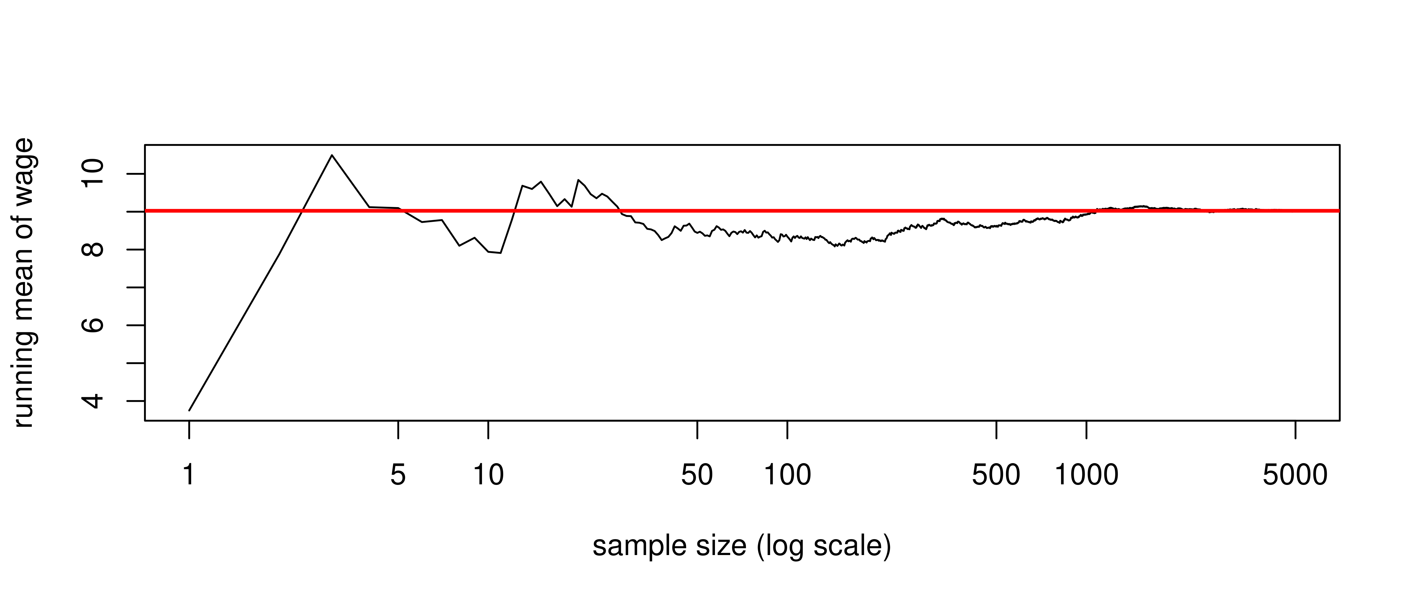
\bar X_n \;\overset{p}{\longrightarrow}\; E(X) \qquad\text{i.e.}\qquad \mathrm{plim}_{n\to\infty} \bar X_n = E(X)
\hat\theta_n is consistent for \theta if \mathrm{plim}_{n\to\infty}\hat\theta_n = \theta.
Under MLR.1–MLR.4, OLS is consistent. For simple regression the argument is three lines:
\hat\beta_1 = \beta_1 + \frac{n^{-1}\sum_i (X_i - \bar X)U_i}{n^{-1}\sum_i (X_i - \bar X)X_i} \;\overset{p}{\longrightarrow}\; \beta_1 + \frac{\mathrm{Cov}(X, U)}{\mathrm{Var}(X)}
So consistency needs only \mathrm{Cov}(X, U) = 0 — weaker than SLR.4’s E(U\mid X) = 0.
Clive Granger: “If you cannot get it right as n goes to infinity, you shouldn’t be in this business.”
##      n   mean     sd sd_x_sqrt_n
## 1   25 0.0745 0.0399      0.1994
## 2   50 0.0749 0.0286      0.2020
## 3  100 0.0766 0.0198      0.1978
## 4  250 0.0771 0.0121      0.1911
## 5  500 0.0774 0.0080      0.1789
## 6 1000 0.0766 0.0058      0.1835
## 7 5000 0.0767 0.0028      0.1995
The mean sits on \beta_1 = 0.0768 at every n (unbiasedness), and the spread collapses to zero (consistency). Note the last column: \sqrt{n}\,\mathrm{sd}(\hat\beta_1) is roughly constant, which is exactly the object the CLT describes.
The same plim formula reads as a warning:
\mathrm{plim}\,\hat\beta_1 = \beta_1 + \frac{\mathrm{Cov}(X_1, \varepsilon)}{\mathrm{Var}(X_1)} = \beta_1 + \beta_2 \frac{\mathrm{Cov}(X_1, X_2)}{\mathrm{Var}(X_1)}
If a confounder is omitted, the estimator converges to the wrong number. It is inconsistent.
More data does not help. It just makes you more confident about something false — the confidence interval shrinks around the wrong value.
This is the single most important asymmetry in econometrics: noise shrinks with n, bias does not.
For an i.i.d. sample with finite variance,
\sqrt{n}\,\big(\bar X_n - E(X)\big) \;\overset{d}{\longrightarrow}\; \mathcal{N}\big(0, \mathrm{Var}(X)\big)
No matter what the distribution of X is.
Applied to OLS: under MLR.1–MLR.5 (note: no MLR.6),
\sqrt{n}\,(\hat\beta_j - \beta_j) \;\overset{d}{\longrightarrow}\; \mathcal{N}\!\left(0, \frac{\sigma^2}{a_j^2}\right), \qquad a_j^2 = \mathrm{plim}\; n^{-1}\sum_i \hat r_{ij}^2
and therefore
T = \frac{\hat\beta_j - \beta_j}{\mathrm{se}(\hat\beta_j)} \;\overset{a}{\sim}\; \mathcal{N}(0,1)
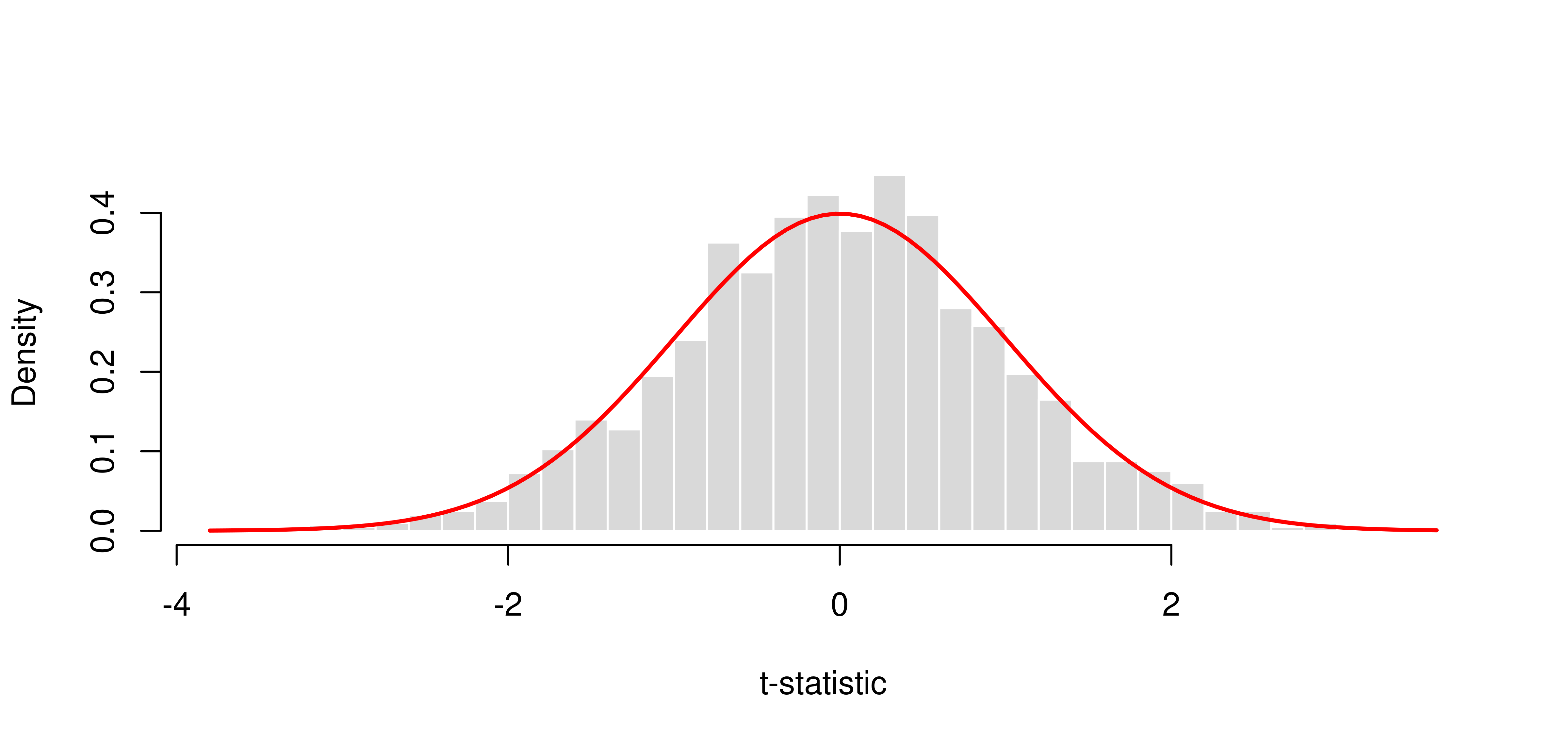
Errors drawn from a shifted exponential: skewed, one-sided, nothing like a normal.
set.seed(4354)
tstat <- replicate(2000, {
  i <- sample(length(educ), 200, replace = TRUE)
  u <- (rexp(200) - 1) * sig                      # mean 0, strongly skewed
  y <- beta[1] + beta[2] * educ[i] + u
  s <- summary(lm(y ~ educ[i]))
  (s$coefficients[2, 1] - beta[2]) / s$coefficients[2, 2]
})
c(mean = mean(tstat), sd = sd(tstat))
## mean sd
## 0.005686162 1.001061572MLR.6 was violated as badly as we could manage, and the t-statistic is still standard normal.
Buys: we can drop MLR.6 entirely. Confidence intervals, t-tests, and F-tests are computed exactly as before.
Costs: every statement becomes an approximation.
| small n | large n | |
|---|---|---|
| U \sim \mathcal{N}(0,\sigma^2) | T \sim t_{n-k-1} exactly | T \approx \mathcal{N}(0,1) |
| U distribution unknown | nothing | T \approx \mathcal{N}(0,1) |
Everything so far judged an estimator by how close \hat\beta is to \beta.
For forecasting, we do not care about \beta much (not always). We care about how close \hat Y^* is to Y^* for a unit we have not seen.
E\big[(Y^* - \hat Y^*)^2\big] = \underbrace{\sigma^2}_{\text{irreducible}} + \underbrace{\big(E\hat Y^* - E(Y^*\!\mid\! x^*)\big)^2}_{\text{bias}^2} + \underbrace{\mathrm{Var}(\hat Y^*)}_{\text{variance}}
That middle term is why BLUE stops being the right target: a little bias can be worth a lot of variance.
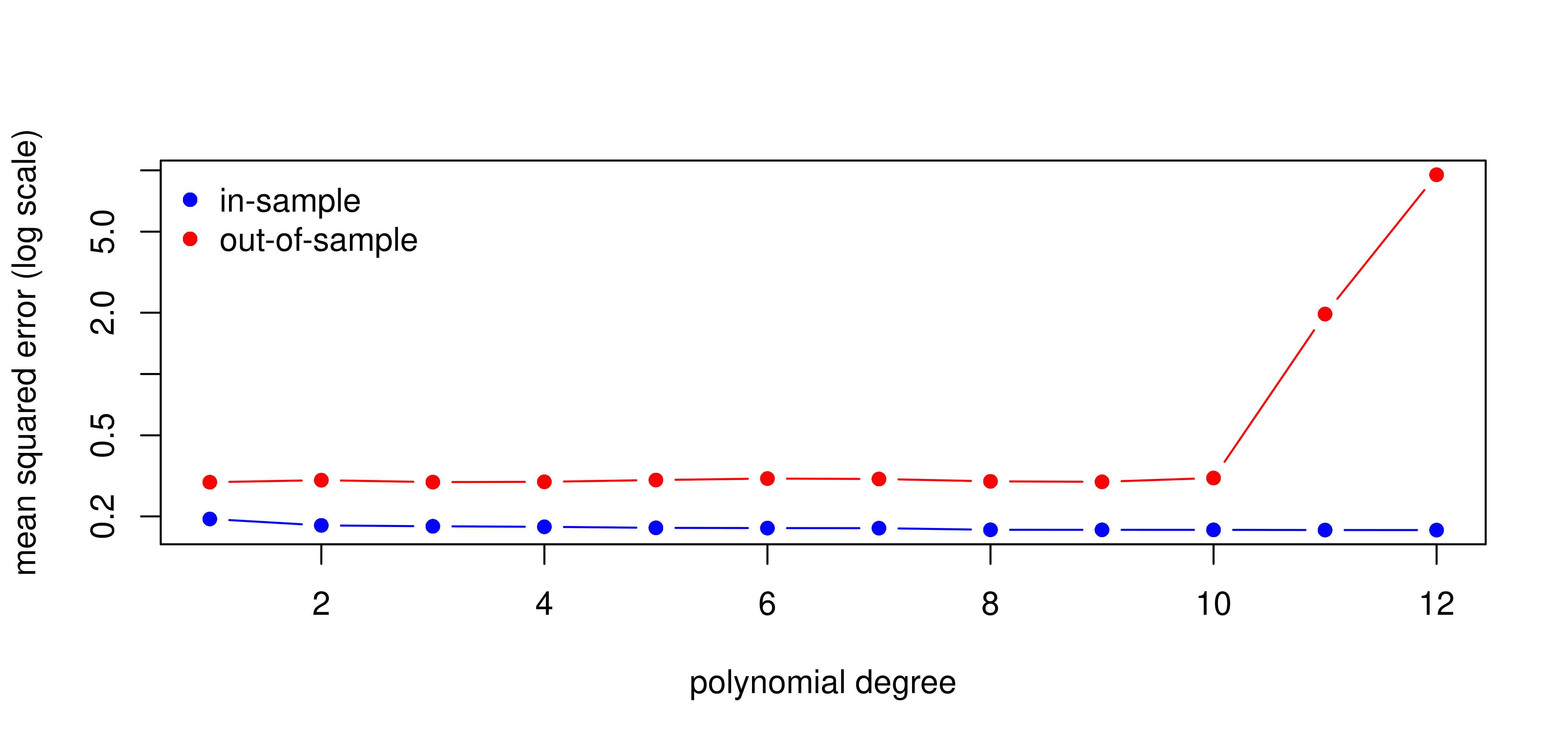
Split the sample: fit on 400 workers, evaluate on the held-out 134.
set.seed(1)
train <- sample(nrow(cps), 400)
mse <- sapply(1:12, function(p) {
  f <- lm(lwage ~ poly(education, p) + poly(experience, p), data = cps[train, ])
  c(in_sample  = mean(resid(f)^2),
    out_sample = mean((cps$lwage[-train] -
                       predict(f, newdata = cps[-train, ]))^2))
})
round(t(mse)[c(1, 3, 6, 9, 10, 11, 12), ], 4)
## in_sample out_sample
## [1,] 0.1943 0.2944
## [2,] 0.1788 0.2947
## [3,] 0.1752 0.3067
## [4,] 0.1718 0.2956
## [5,] 0.1718 0.3087
## [6,] 0.1714 1.9694
## [7,] 0.1713 9.5127In-sample error falls forever. Out-of-sample error explodes.
The three problems this session set up, and what we do about them:
Same machinery. Different question.
| Object | Formula |
|---|---|
| OLS slope | \hat\beta_1 = \widehat{\mathrm{Cov}}(X,Y)/\widehat{\mathrm{Var}}(X) |
| Residual algebra | \sum_i \hat U_i = 0, \sum_i X_i \hat U_i = 0 |
| Decomposition | SST = SSE + SSR; R^2 = SSE/SST |
| Adjusted R^2 | \bar R^2 = 1 - (1-R^2)\frac{n-1}{n-k-1} |
| Unbiasedness | MLR.1–4 \Rightarrow E(\hat\beta_j) = \beta_j |
| Variance | \mathrm{Var}(\hat\beta_j) = \sigma^2 / [SST_j (1-R_j^2)] |
| Gauss–Markov | MLR.1–5 \Rightarrow OLS is BLUE |
| OVB | \tilde\beta_1 = \hat\beta_1 + \hat\beta_2 \tilde\delta_1 |
| Partialling out | \hat\beta_j = \sum_i \hat r_{ij} Y_i / \sum_i \hat r_{ij}^2 |
| t-statistic | T = (\hat\beta_j - a)/\mathrm{se}(\hat\beta_j) \sim t_{n-k-1} under MLR.1–6 |
| F-statistic | F = \frac{(SSR_r - SSR_{ur})/q}{SSR_{ur}/(n-k-1)} \sim F_{q,\,n-k-1} |
| Asymptotics | MLR.1–5 \Rightarrow T \overset{a}{\sim} \mathcal{N}(0,1), no MLR.6 needed |
fit <- lm(y ~ x1 + x2, data = df)   # fit
summary(fit)                        # coefficients, se, t, p, R2, overall F
coef(fit); resid(fit); fitted(fit)  # extract
confint(fit, level = 0.95)          # confidence intervals
predict(fit, newdata = new_df)      # forecast
anova(restricted, unrestricted)     # F-test for exclusion restrictions
car::linearHypothesis(fit, "x1 - x2 = 0")   # general linear restriction
car::vif(fit)                       # multicollinearity diagnostics
lm(y ~ x1 * x2, data = df)          # x1 + x2 + x1:x2
lm(y ~ x1 + I(x1^2), data = df)     # I() protects arithmetic in a formula
lmtest::coeftest(fit, vcov = sandwich::vcovHC) # heteroskedasticity-robust seAER::CPS1985 — the running example. data("CPS1985") after library(AER); ?CPS1985 for the codebook.wooldridge package ships every dataset from the textbook: install.packages("wooldridge").