In R, we do things using functions, as soon as we use it beyond a calculator.
Modularity: break a complex problem into small, manageable pieces. During development you focus on one function at a time instead of the whole project.
Scope management: functions provide local scope. Objects created inside a function stay inside it; only inputs and outputs touch the global environment.
Reusability, the DRY principle: “Don’t Repeat Yourself”. When something changes, you edit one definition instead of the same code in ten places.
Calling functions
We have already seen and used a multitude of functions in R.
Some come pre-packaged with base R (e.g. mean())
Others come from external packages (e.g. mvtnorm::rmvnorm())
Regardless of where they come from, functions in R all adopt the same basic syntax:
function_name(ARGUMENTS)
Writing your own functions
Most of the time we rely on functions that other people have written for us. But you can, and should, write your own too, with the generic function() function.1
function(ARGUMENTS) { OPERATIONSreturn(VALUE)}
1 Yes, it is a function that lets you write functions. Very meta.
Name your functions
Writing anonymous functions like the above is possible and reasonably common. But we typically write functions because we want to reuse code, and for that it makes sense to name them.1
Short functions need neither the curly brackets nor an explicit return object, so you can write them on a single line:
my_short_func =function(ARGUMENTS) OPERATION
1 Remember: “In R, everything is an object and everything has a name.”
Name your functions (cont.)
Tip
Try to give your functions short, pithy names that are informative to both you and anyone else reading your code. This is harder than it sounds, but will pay off down the road.
Two things we still owe you, and which the next few slides deliver:
when the curly brackets and the explicit return() actually matter;
what happens to the objects created inside the brackets.
Simple example: addition
# Built-in functionsum(c(3, 4))
## [1] 7
# User-defined functionadd_func <-function(x, y) { total <- x + y ## Create an intermediary object (that will be returned)return(total) ## The value(s) or object(s) that we want returned.}add_func(3, 4)
## [1] 7
Return explicitly
Caution
R’s default behaviour is to automatically return the final object that you created within the function. However, this won’t always be the case. Get into the habit of assigning the return object(s) explicitly.
An explicit return() is also how we hand back more than one object:
add_func <-function(x, y) { total <- x + yreturn(list(sum = total, first_element = x, second_element = y))}add_func(3, 4)
None of the intermediate objects created inside the functions above (total, etc.) made their way into our global environment. Confirm this in the “Environment” pane of RStudio.
R has a set of lexical scoping rules governing where it stores and evaluates the values of different objects.
Functions operate in a quasi-sandboxed environment.
They do not return or use objects in the global environment unless forced to, e.g. by a return() command.
A function only looks to outside environments, e.g. a level “up”, if it does not see the object named within itself.
Example: OLS estimation
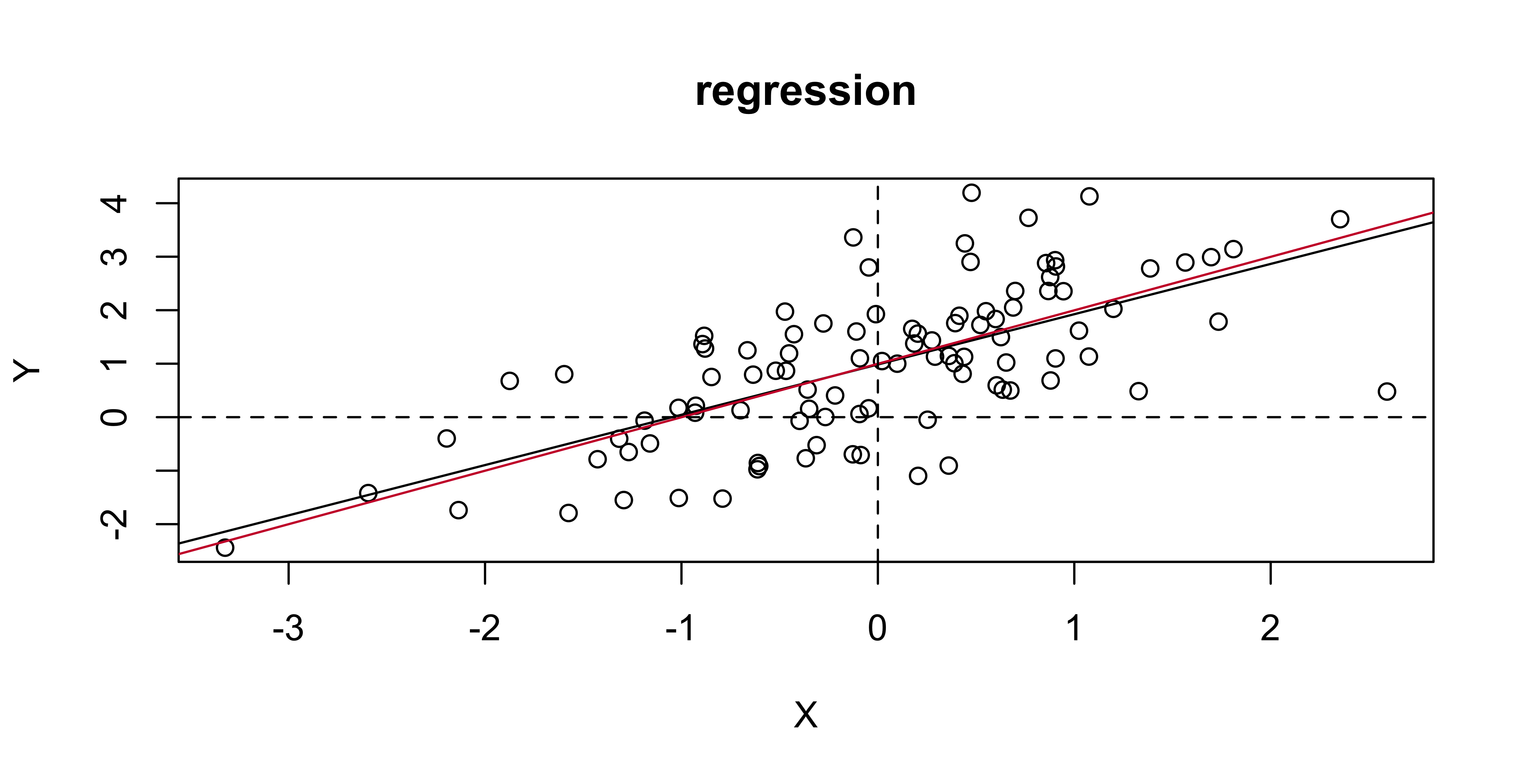
Consider a simple linear regression model with a constant term and one regressor:
y_i = \beta_0 + \beta_1 x_i + \varepsilon_i
y_i: the dependent variable
x_i: the independent variable
\beta_0: the intercept, \beta_1: the slope coefficient
To conduct OLS estimation in R, we literally translate this mathematical expression into code.
Step 1: simulate the data
We need data Y and X to run OLS, so we simulate an artificial dataset.
# simulate dataset.seed(111) # can be removed to allow the result to change# set the parametersn <-100b0 <-matrix(1, nrow =2)# generate the datae <-rnorm(n)X <-cbind(1, rnorm(n))Y <- X %*% b0 + e
Step 1: simulate the data (cont.)
# Snapshot of X (first 10 rows):print(head(X, 10))
Jim Hester’s lookup package does the legwork for you
Packages
R’s package ecosystem
A base R installation is relatively compact. R’s true power lies in its extensive ecosystem of add-on packages, most of them hosted on CRAN, the Comprehensive R Archive Network.
A common practice in the statistical community: researchers publish an R package alongside the academic paper.
New statistical methods become immediately accessible to practitioners.
A virtuous cycle: researchers gain visibility, users get cutting-edge tools within months, sometimes weeks, of publication.
Install and load packages
A package is installed by install.packages("package_name") and invoked by library(package_name).
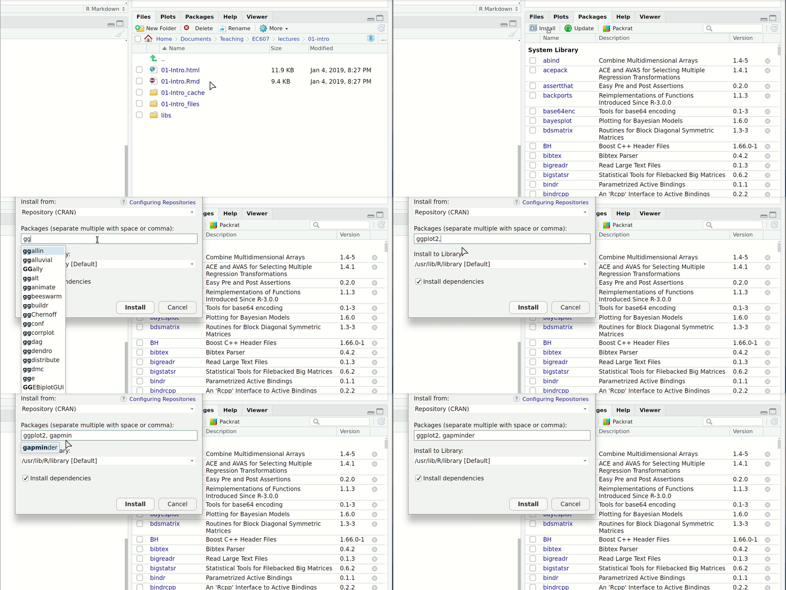
To install ggplot2, either:
Console: enter install.packages("ggplot2").
RStudio: click the “Packages” tab in the bottom-right pane, then “Install”, and search for the package.
Install and load packages (cont.)
Loading packages
Once installed, load a package into your R session with library().
library(ggplot2)
Note
Notice that you do not need quotes around the package name any more.
Reason: R now recognizes the package as a defined object with a given name. (“Everything in R is an object and everything has a name.”)
Shortcuts and namespaces
Tip
A convenient way to combine installation and loading is the pacman package’sp_load() function. pacman::p_load(ggplot2) first checks whether it needs to install the package, then loads it. Clever.
We can also run a function from an installed package without loading it, using PACKAGE::package_function():
stats::sd(1:10)
## [1] 3.02765
Packages beyond CRAN
Many authors distribute packages through GitHub or their personal websites, especially for cutting-edge research or development versions.
Install them with devtools or remotes.
Follow the instructions on the project’s repository, e.g. RDHonest.
if (!requireNamespace("remotes")) {install.packages("remotes")}remotes::install_github("kolesarm/RDHonest")
A modern approach to developing R packages is through literate programming.
The litr package, by Jacob Bien, lets you write a complete R package inside a single R Markdown document.
The package is created when you knit the Rmd file.
For larger packages, you can write a bookdown that defines the package.
Interested? The videos show how it works in a few minutes.
Control Flow
Controlling the flow
Now that we have a good sense of the basic function syntax, it is time to learn control flow: controlling the order, or “flow”, of the statements and operations that our functions evaluate.
This is common to all programming languages.
if is used for choice.
for and while are used for loops.
if
The basic syntax for an if statement:
if (CONDITION) { OPERATION}
square_root <-function(x) {if (x <0) {message("x is negative")return(NA) }return(sqrt(x))}square_root(9)
## [1] 3
square_root(-9)
## x is negative
## [1] NA
if ... else
We can extend this with an else statement to handle alternative conditions:
To guard against this behaviour, and to add some other optimisations, both the tidyverse (through dplyr) and data.table offer their own versions of ifelse.
As you may have guessed, it is certainly possible to write nested ifelse() statements:
ifelse(CONDITION1, DO IF TRUE, ifelse(CONDITION2, DO IF TRUE, ifelse(...)))
or
if (CONDITION1) { DO IF TRUE} elseif (CONDITION2) { DO IF TRUE} else { DO IF FALSE}
However, these nested statements quickly become difficult to read and troubleshoot.
case when
A better solution was originally developed in SQL with the CASE WHEN statement. Both dplyr (case_when()) and data.table (fcase()) provide implementations in R.
x <-1:10## dplyr::case_when()case_when( x <=3~"small", x <=7~"medium",TRUE~"big"## Default value. Could also write `x > 7 ~ "big"` here.)
When we use loops, we should minimize the tasks within the loop.
Pre-specify the dimension and allocate memory for variables outside the loop.
In cases where we want to “grow” an object via a for loop, we first have to create an empty (or NULL) object, and R re-allocates memory at every iteration.
Let us measure how much this actually costs.
Example: empirical coverage of a confidence interval
CI <-function(x) {# construct confidence interval# x is a vector of random variables n <-length(x) mu <-mean(x) sig <-sd(x) upper <- mu +1.96/sqrt(n) * sig lower <- mu -1.96/sqrt(n) * sigreturn(list(lower = lower, upper = upper))}Rep <-100000sample_size <-1000mu <-2
Option 1: append a new outcome after each loop
pts0 <-Sys.time() # check timefor (i in1:Rep) { x <-rpois(sample_size, mu) bounds <-CI(x) out_i <- ((bounds$lower <= mu) & (mu <= bounds$upper))if (i ==1) { out <- out_i } else { out <-c(out, out_i) }}mean(out)
## [1] 0.95023
cat("Takes", Sys.time() - pts0, "seconds\n")
## Takes 7.249099 seconds
Option 2: initialize the result vector
# Initialize the result vectorout <-rep(0, Rep)pts0 <-Sys.time() # check timefor (i in1:Rep) { x <-rpois(sample_size, mu) bounds <-CI(x) out[i] <- ((bounds$lower <= mu) & (mu <= bounds$upper))}mean(out)
## [1] 0.94893
cat("Takes", Sys.time() - pts0, "seconds\n")
## Takes 2.395516 seconds
Identical answer, and the empirical coverage sits close to the nominal 95%. Pre-allocating is the cheaper route.
Vectorization
Before we write any loops, we should ask ourselves: “Do I need to iterate at all?”
R is vectorized. Often you can apply a function to every element of a vector at once, rather than one at a time.
In R and other high-level languages, for loops can be slow. When you loop through many elements and perform an expensive operation on each one, your code may take a long time to execute.
Many operations typically implemented with for-loops can be rewritten using vectorized operations or matrix computations.
Whenever possible, leverage R’s built-in vectorization capabilities for better performance.
Functional programming (FP) is arguably the most important thing you can take away from today’s lecture. Hadley Wickham puts the core idea like this in Advanced R:
R, at its heart, is a functional programming (FP) language. […] R has what’s known as first class functions.
You can do anything with a function that you can do with a vector:
assign it to a variable,
store it in a list,
pass it as an argument to another function,
create it inside a function,
return it as the result of a function.
Hadley explains it better
Why not for loops?
Summary:for loops emphasise the objects we are working with (say, a vector of numbers) rather than the operations we want to apply to them (get the mean, or the median, or whatever).
This is inefficient: it requires us to write out the for loop by hand rather than getting an R function to create the loop for us.
As a corollary, for loops pollute our global environment with counting variables. Look at your “Environment” pane: i is sitting there, equal to the last value of its loop.
Creating those auxiliary variables is almost certainly not an intended outcome, and they can cause errors when we inadvertently refer to a similarly-named variable elsewhere in our script. So we best remove them as soon as we are finished.
rm(i)
Why not for loops? (cont.)
Another annoyance arrived in cases where we want to “grow” an object as we iterate over it. To do that with a for loop, we had to create an empty object first.
FP lets us avoid the explicit loop construct and its associated downsides. In practice, there are two ways to implement FP in R:
No i in your global environment. Because of R’s lexical scoping rules, any object created and invoked by a function is evaluated in a sandbox outside your global environment.
The syntax barely changed when switching from for() to lapply(). The essential structure is the same: first the iteration list (1:10), then the desired function or operation (LETTERS[i]).
The returned object is a list.lapply() accepts vectors, data frames and lists as arguments, but always returns a list, with one element per iteration of the loop. (So now you know where the “l” in “lapply” comes from.)
Getting output that is not a list
Several options exist.1 The one I use most commonly is to bind the list elements into a single data frame with dplyr::bind_rows() or data.table::rbindlist().
lapply(1:10, function(i) { df <-tibble(num = i, let = LETTERS[i])return(df)}) %>%bind_rows()
## # A tibble: 10 × 2
##      num let
##    <int> <chr>
##  1     1 A
##  2     2 B
##  3     3 C
##  4     4 D
##  5     5 E
##  6     6 F
##  7     7 G
##  8     8 H
##  9     9 I
## 10    10 J
1 E.g. pipe the output to unlist() if you want a vector, or use sapply(), which is covered next.
Why lapply() anyway?
The default list-return behaviour may not sound ideal at first, but I use lapply() more frequently than any of the other apply family members.
My functions normally return multiple objects of different type, which makes a list the only sensible format;
or they return a single data frame, which is where dplyr::bind_rows() and data.table::rbindlist() come in.
The *apply family: sapply()
sapply() stands for “simplify apply”. It is essentially a wrapper around lapply that tries to return simplified output that matches the input type. Feed it a vector and it will try to return a vector.
sapply(1:10, function(i) LETTERS[i])
## [1] "A" "B" "C" "D" "E" "F" "G" "H" "I" "J"
The *apply family: apply()
apply() applies functions over array margins: the rows or columns of matrices and data frames.
# Create a simple matrixmat <-matrix(1:12, nrow =3, ncol =4)print(mat)
For a concise overview of the different *apply() functions, see this blog post by Neil Saunders.
2) The purrr package
purrr’s map() is the tidyverse’s lapply(). Same syntax, same list output:
map(1:10, function(i) { ## only need to swap `lapply` for `map` df <-tibble(num = i, let = LETTERS[i])return(df)})
## [[1]]
## # A tibble: 1 × 2
##     num let
##   <int> <chr>
## 1     1 A
##
## [[2]]
## # A tibble: 1 × 2
##     num let
##   <int> <chr>
## 1     2 B
##
## [[3]]
## # A tibble: 1 × 2
##     num let
##   <int> <chr>
## 1     3 C
##
## [[4]]
## # A tibble: 1 × 2
##     num let
##   <int> <chr>
## 1     4 D
##
## [[5]]
## # A tibble: 1 × 2
##     num let
##   <int> <chr>
## 1     5 E
##
## [[6]]
## # A tibble: 1 × 2
##     num let
##   <int> <chr>
## 1     6 F
##
## [[7]]
## # A tibble: 1 × 2
##     num let
##   <int> <chr>
## 1     7 G
##
## [[8]]
## # A tibble: 1 × 2
##     num let
##   <int> <chr>
## 1     8 H
##
## [[9]]
## # A tibble: 1 × 2
##     num let
##   <int> <chr>
## 1     9 I
##
## [[10]]
## # A tibble: 1 × 2
##     num let
##   <int> <chr>
## 1    10 J
map_df(): pick your output type
map() comes with its own variants for returning objects of a desired type. purrr::map_df() returns a data frame:
map_df(1:10, function(i) { ## don't need bind_rows with `map_df` df <-tibble(num = i, let = LETTERS[i])return(df)})
## # A tibble: 10 × 2
##      num let
##    <int> <chr>
##  1     1 A
##  2     2 B
##  3     3 C
##  4     4 D
##  5     5 E
##  6     6 F
##  7     7 G
##  8     8 H
##  9     9 I
## 10    10 J
More efficient, i.e. less typing, than the lapply() version: no extra row-binding step at the end. Jenny Bryan’s purrr tutorial goes much deeper.
Create and iterate over named functions
We can split the function and the iteration (and binding) into separate steps. This is generally a good idea, since you typically create named functions with the goal of reusing them.
## Create a named functionnum_to_alpha <-function(i) { df <-tibble(num = i, let = LETTERS[i])return(df) }
Create and iterate over named functions (cont.)
Now we can easily iterate over our function using different input values.
lapply(1:10, num_to_alpha) %>%bind_rows()
## # A tibble: 10 × 2
##      num let
##    <int> <chr>
##  1     1 A
##  2     2 B
##  3     3 C
##  4     4 D
##  5     5 E
##  6     6 F
##  7     7 G
##  8     8 H
##  9     9 I
## 10    10 J
map_df(c(1, 5, 26, 3), num_to_alpha)
## # A tibble: 4 × 2
##     num let
##   <dbl> <chr>
## 1     1 A
## 2     5 E
## 3    26 Z
## 4     3 C
R Markdown and Quarto
R Markdown
A document format that combines the power of R programming with the simplicity of Markdown syntax. Code, results, and narrative text coexist seamlessly.
R Markdown provides an authoring framework for data science. You can use a single R Markdown file to both
save and execute code
generate high quality reports that can be shared with an audience
Key features of R Markdown
Reproducible research: your analysis and results are automatically updated when you change your code or data.
Multiple output formats: HTML, PDF, Word documents, presentations and more, all from the same source.
Code integration: embed R code chunks that execute and display results inline with your text.
Version control friendly: the plain text format works well with Git and other version control systems.
Basic structure
An R Markdown document consists of three main components:
YAML header: metadata and output options, enclosed by ---
Markdown text: regular text formatted with Markdown syntax
Code chunks: R code blocks enclosed by triple backticks with {r}
This deck, and the long-form note it mirrors, are themselves such documents.
Code chunks
Code chunks are the heart of R Markdown. They allow you to:
execute R code and display results;
control output with chunk options, e.g. echo=FALSE, eval=FALSE;