ECON 4354 / 6354 Forecasting

Lecture 0: Course Overview

Zhan Gao

25 August 2026

Overview

1. Introduction
2. Syllabus
3. Software Installation
4. R Basics

Introduction

Instructor

Zhan Gao (website)
zhangao [at] smu [dot] edu
Office Hours: Tuesday and Thursday 4 - 5pm @ 301U, Umphrey Lee

Teaching Assistant

Furong Guo
furongg [at] smu [dot] edu
Office Hours: Tuesday and Thursday 2 - 4pm by appointment

Syllabus Highlights

---

(Read the full document on Canvas.)

Learning Outcomes

• Understand the fundamental properties of time series data

• Understand the fundamental modeling techniques for time series

• Implement econometric methods and machine learning algorithms for economic forecasting

Observations over time

• Natural ordering of observations

• A single realization in history

• Macroeconomic applications
  • FRED database
• Financial applications
  • Yahoo Finance

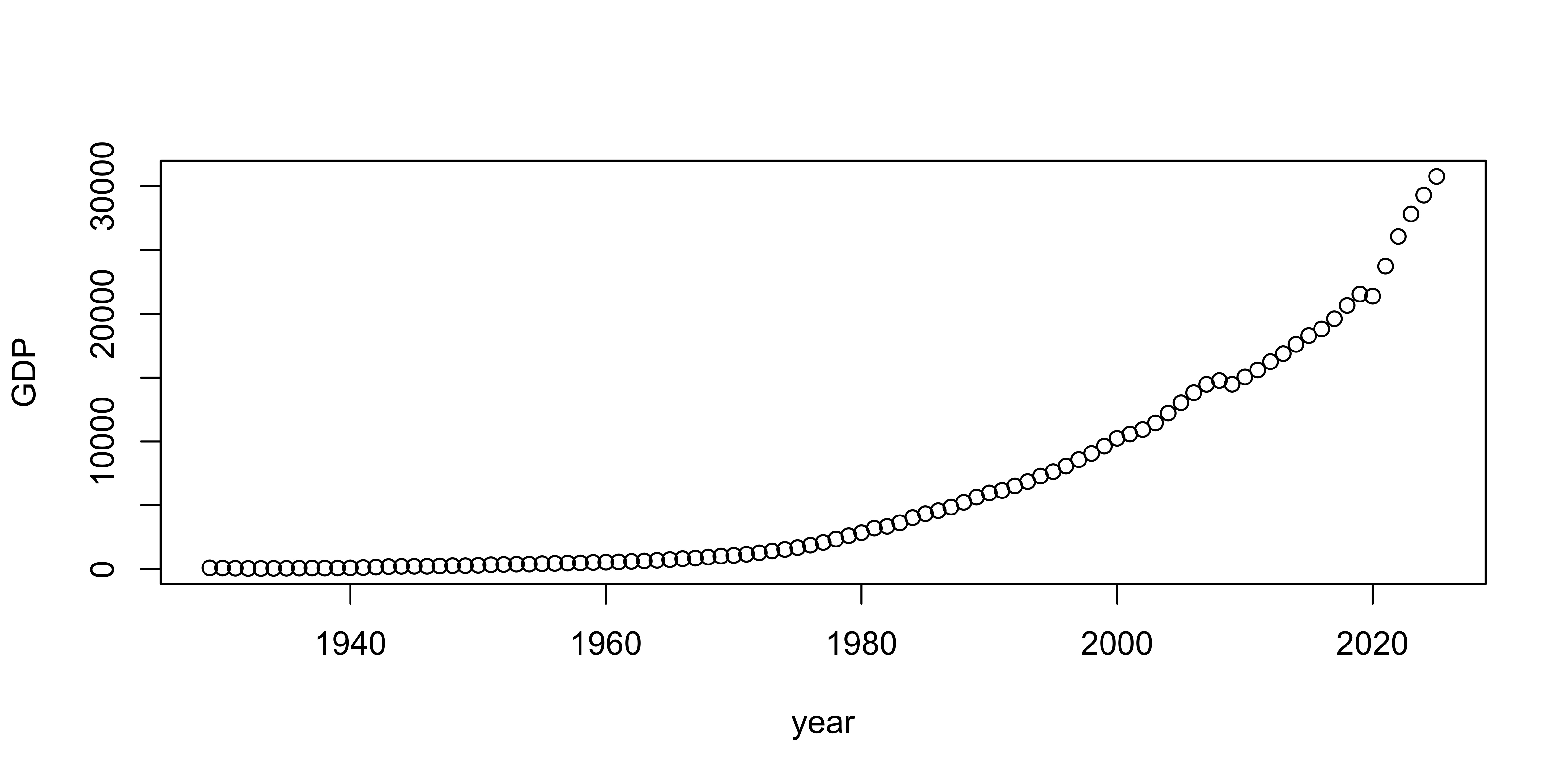
US GDP

USA <- read.csv("https://fred.stlouisfed.org/graph/fredgraph.csv?id=GDPA")
USA$observation_date <- as.Date(USA$observation_date)
head(USA, n = 3)

##   observation_date    GDPA
## 1       1929-01-01 104.556
## 2       1930-01-01  92.160
## 3       1931-01-01  77.391

plot(x = USA$observation_date, y = USA$GDPA, xlab = "year", ylab = "GDP")

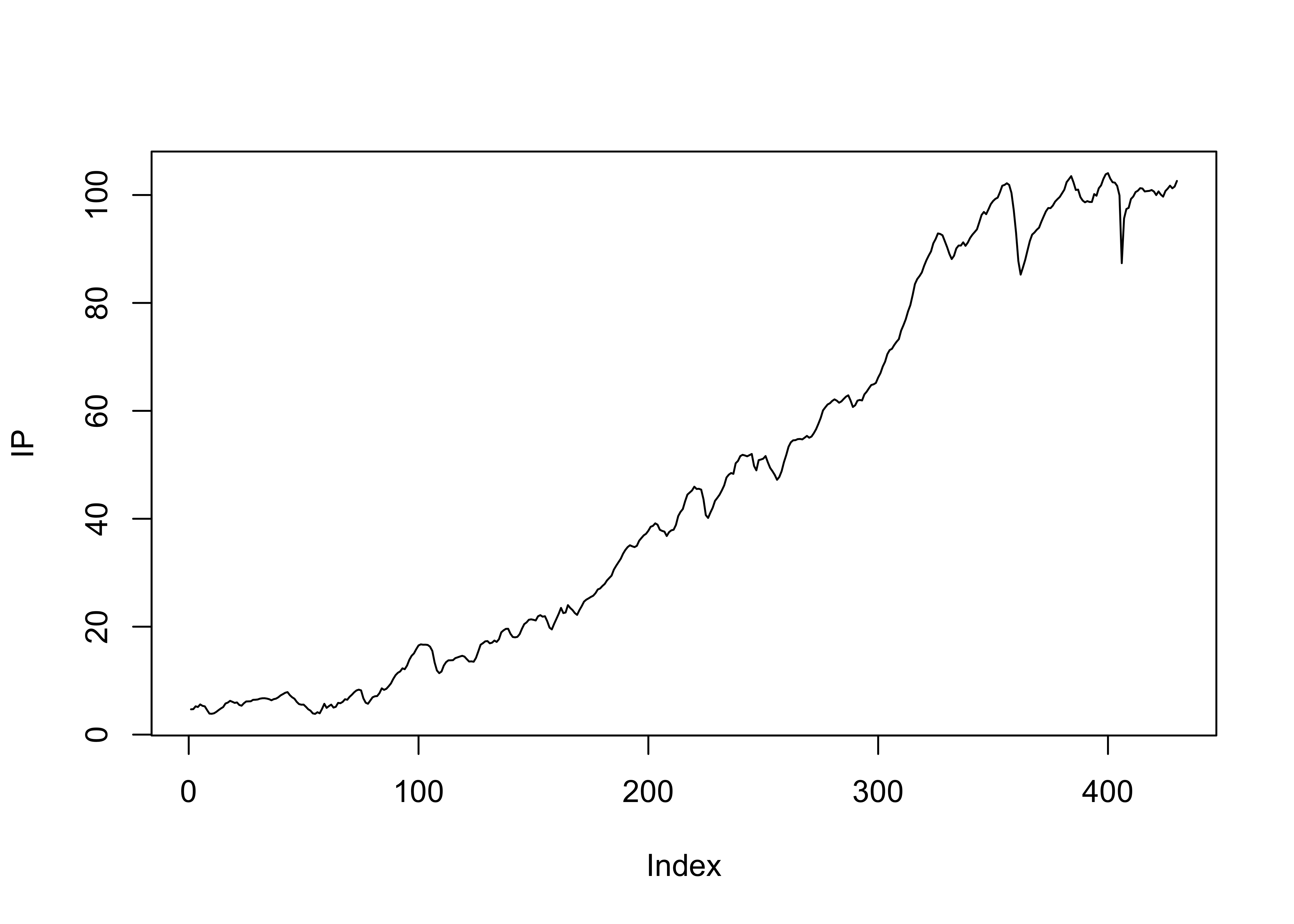
USA Industrial Production

• Another example: Quarterly US Industrial Production Index

IP <- read.csv(paste0(
  "https://fred.stlouisfed.org/graph/fredgraph.csv",
  "?id=IPB50001SQ"))
IP <- xts::xts(IP["IPB50001SQ"],
               as.Date(IP$observation_date))
head(IP, 3)

##            IPB50001SQ
## 1919-01-01     4.6854
## 1919-04-01     4.7213
## 1919-07-01     5.2419

plot(IP, type = "l")

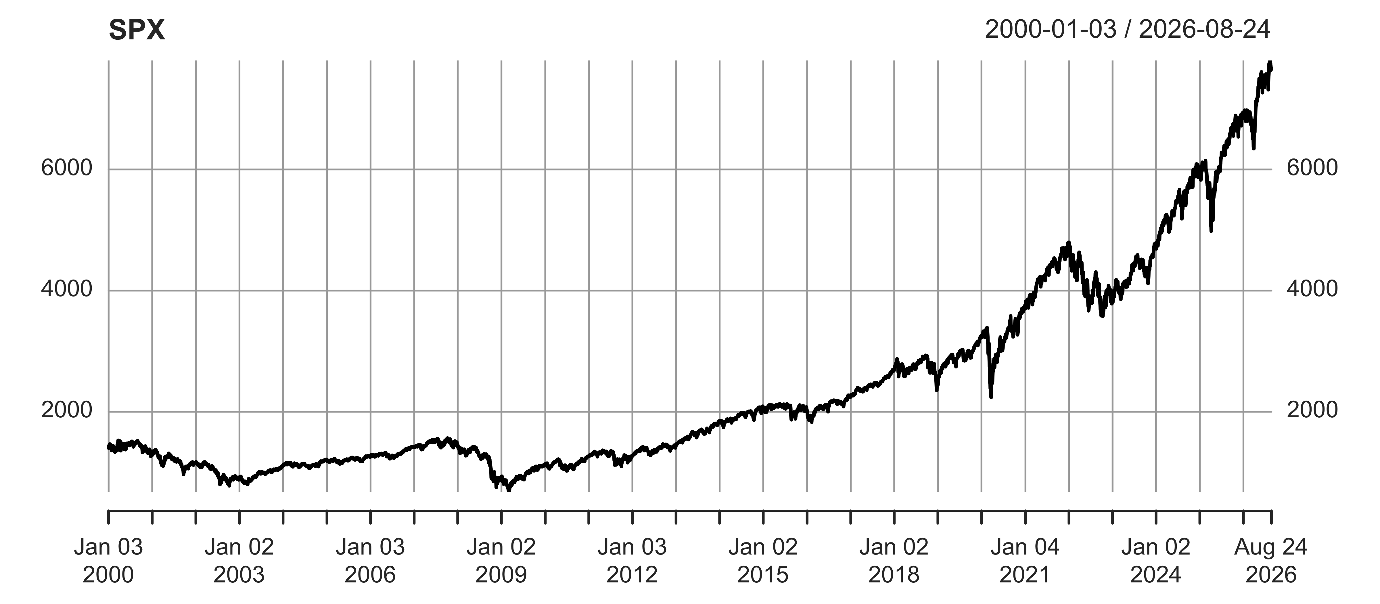
S&P 500 Index

SPX <- quantmod::getSymbols("^GSPC",
                            auto.assign = FALSE, 
                            from = "2000-01-01")$GSPC.Close
plot(SPX)

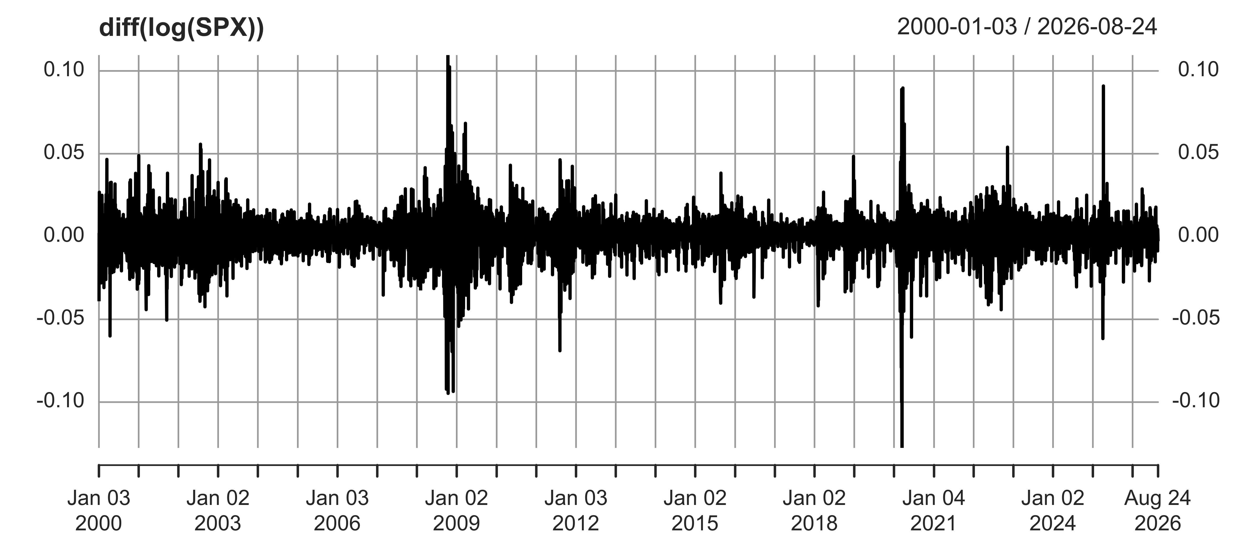
S&P 500 Return

plot( diff( log(SPX) ) )

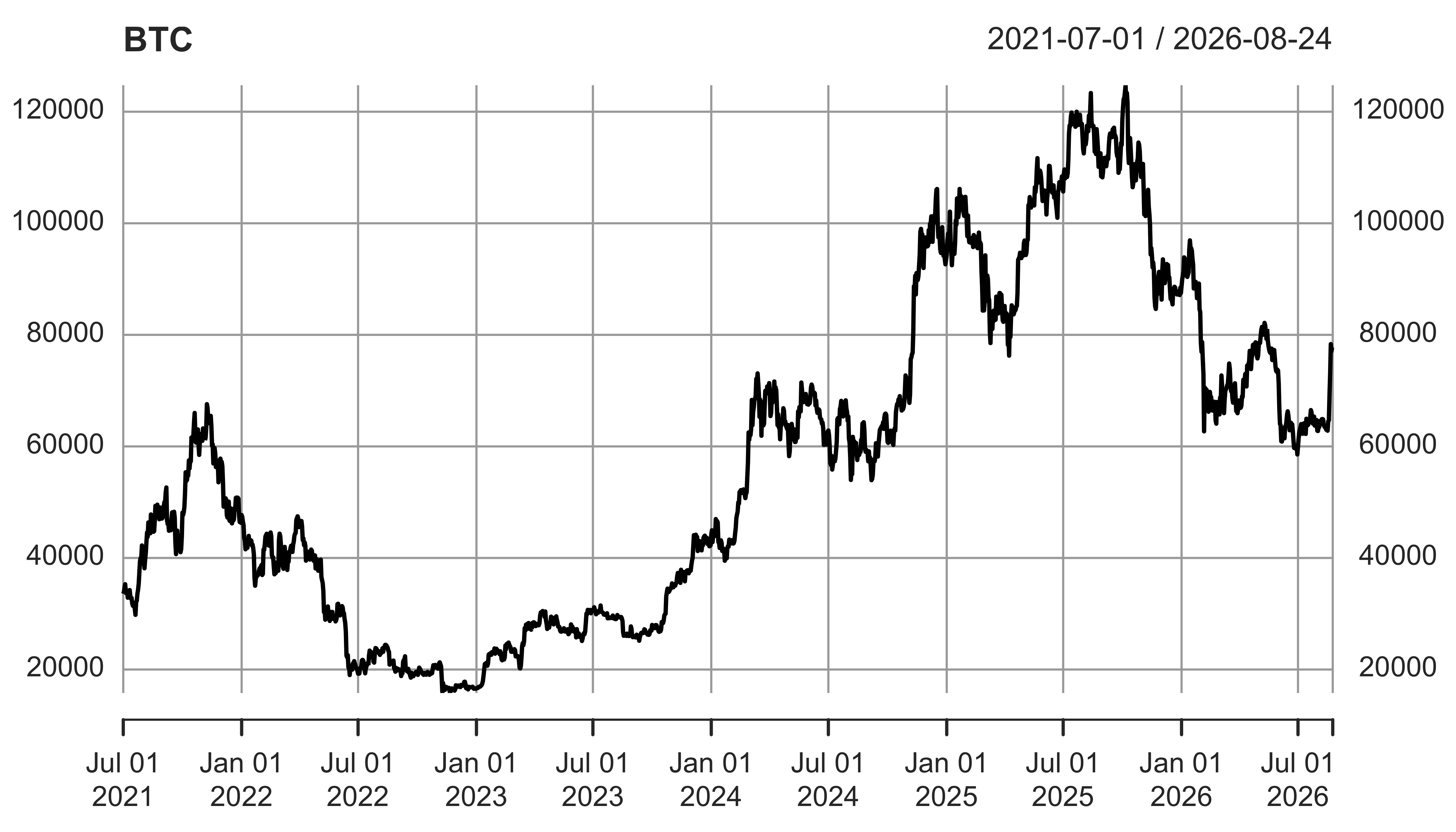
Bitcoin

BTC <- quantmod::getSymbols("BTC-USD", auto.assign = FALSE, 
                            from = "2021-07-01")[,4]
plot(BTC)
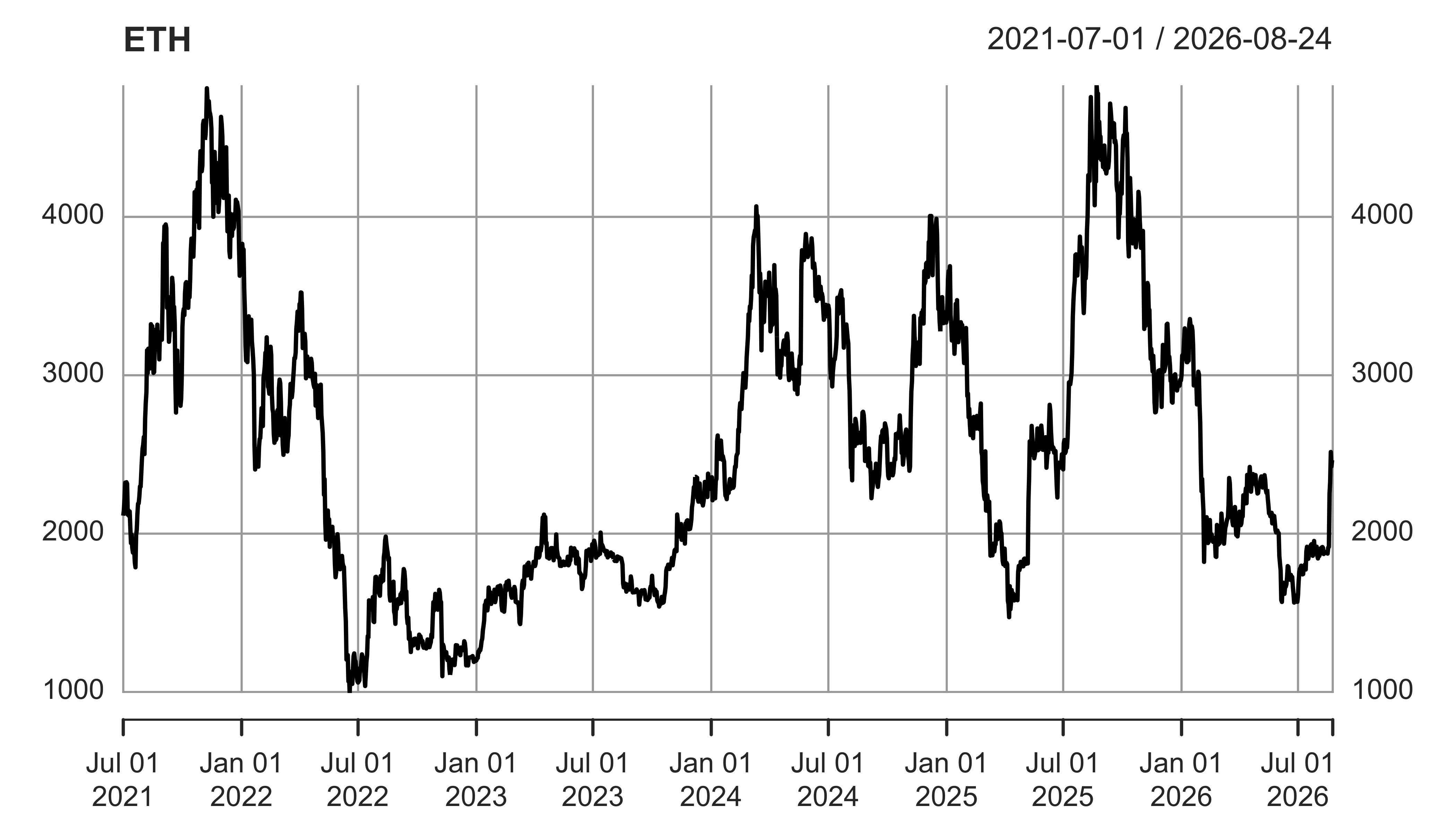
ETH <- quantmod::getSymbols("ETH-USD", auto.assign = FALSE, 
                            from = "2021-07-01")[,4]
plot(ETH)

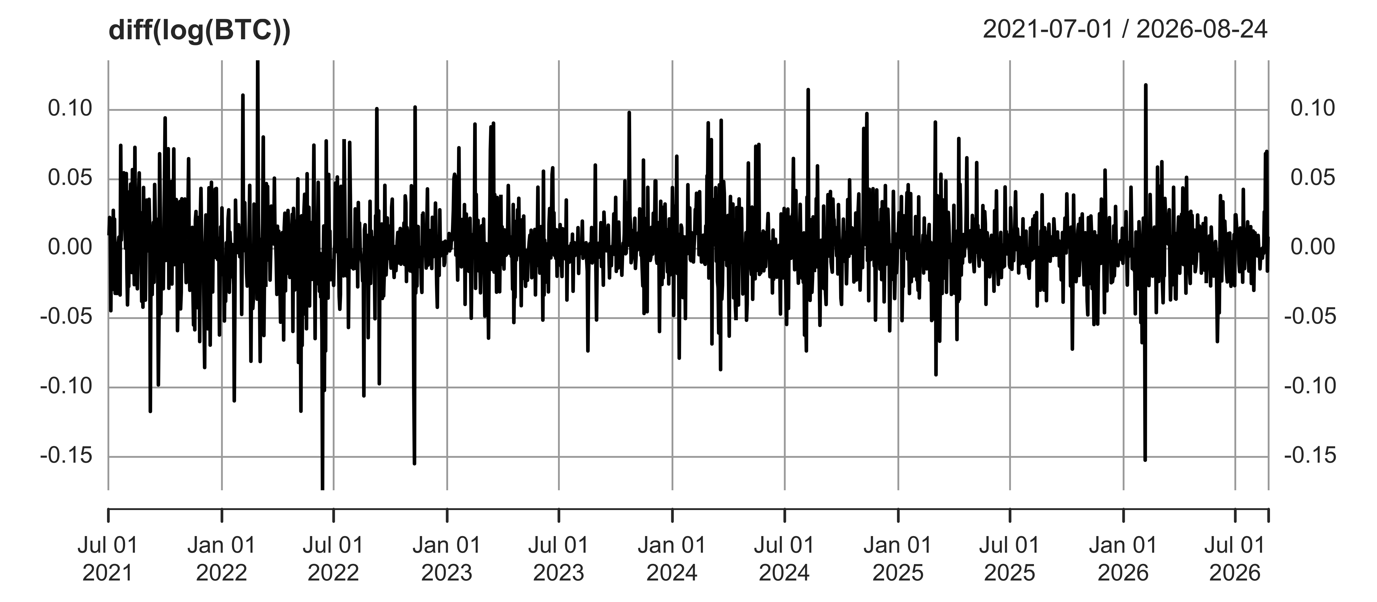
Bitcoin return

plot( diff( log(BTC) ) )

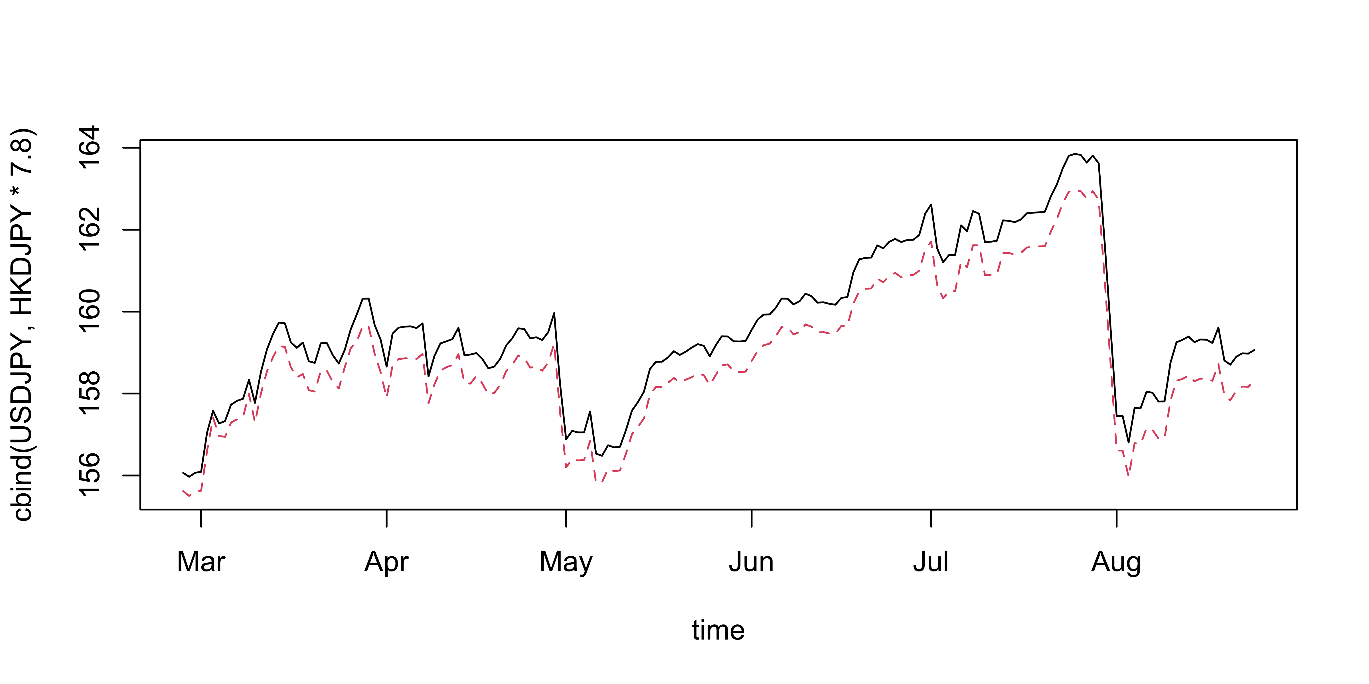
Exchange rates

quantmod::getFX("USD/JPY")

## [1] "USD/JPY"

quantmod::getFX("HKD/JPY")

## [1] "HKD/JPY"

Exchange rates (cont.)

matplot( y = cbind(USDJPY, HKDJPY*7.8), 
         x = zoo::index(USDJPY), type = "l", xlab = "time"  )

Grading policy

Component	Weight
Homework assignments (5% × 4)	20%
In-class exams (25% × 2)	50%
Course project (15% + 15%)	30%

• Everything is posted on, and submitted through, Canvas.

Homework assignments (20%)

Four assignments, each worth 5% of the final grade.

• Due by 11:59pm on September 11, September 25, October 23, and November 6 (all Fridays).

• Assignments are posted on Canvas, and you submit your work in PDF format via Canvas.

• Late submissions will not be accepted.

• Extensions are granted only in cases of documented extenuating circumstances, and must be approved by me before the deadline.

In-class exams (50%)

Two in-class exams, each worth 25% of the final grade.

• Scheduled on October 6 (Tuesday) and November 17 (Tuesday), during our regular class time.

Course project (30%)

Work in groups of two to three to apply the course concepts to a real-world forecasting problem.

• Form a group voluntarily, or wait to be assigned to one after the add/drop period.

Two deliverables, each worth 15%:

1. A final presentation in the last week of class.

2. A final report and replication repository.

Course project: final presentation (15%)

Scheduled on December 3 (Thursday) and December 8 (Tuesday), in the last two classes.

• A 20-minute presentation, followed by a 5-minute Q&A.

Tell the whole story:

1. The project context and the research question.

2. The data and the processing steps.

3. The adopted strategies and the main findings.

4. The policy and/or business implications.

Course project: final report (15%)

Due on December 15 (Tuesday).

• 8–10 pages, including tables, figures, and appendices.

• Self-contained: fully document the context, implementation, analysis, and findings.

• Incorporate the feedback you receive from the presentation.

• Submit a replication repository along with the report, so that anyone can reproduce your results from your code and data.

Getting started

---

Software installation and registration

1. Download R.

2. Download RStudio or Positron.

3. Download Git.

4. Create an account on GitHub and register for a student/educator discount.

• Go-to place for installation guidance and troubleshooting is Jenny Bryan’s http://happygitwithr.com.

Some OS-specific extras

I’ll detail further software requirements as and when the need arises. However, to help smooth some software installation issues further down the road, please also do the following (depending on your OS):

• Windows: Install Rtools. I also recommend that you install Chocolately.
• Mac: Install Homebrew. I also recommend that you configure/open your C++ toolchain (see here.)
• Linux: None (you should be good to go).

Checklist

☑ Do you have the most recent version of R?

version$version.string

## [1] "R version 4.5.3 (2026-03-11)"

☑ Do you have the most recent version of RStudio? (The preview version is fine.)

RStudio.Version()$version
## Requires an interactive session but should return something like "[1] '1.4.1100'"

☑ Have you updated all of your R packages?

update.packages(ask = FALSE, checkBuilt = TRUE)

Checklist (cont.)

Open up the shell.

• Windows users, make sure that you installed a Bash-compatible version of the shell. If you installed Git for Windows, then you should be good to go.

☑ Which version of Git have you installed?

git --version

## git version 2.53.0

☑ Did you introduce yourself to Git? (Substitute in your details.)

git config --global user.name 'Your Name'
git config --global user.email 'your.email@smu.edu'
git config --global --list

☑ Did you register an account in GitHub?

Checklist (cont.)

We will make sure that everything is working properly with your R and GitHub setup next lecture.

For the rest of today’s lecture, I want to go over some very basic R concepts with demonstrations.

About R programming language

---

What is R?

To quote the R project website:

R is a free software environment for statistical computing and graphics. It compiles and runs on a wide variety of UNIX platforms, Windows and MacOS.

What does that mean?

• R was created for the statistical and graphical work required by econometrics.
• R has a vibrant, thriving online community. (stack overflow)
• Plus it’s free and open source.

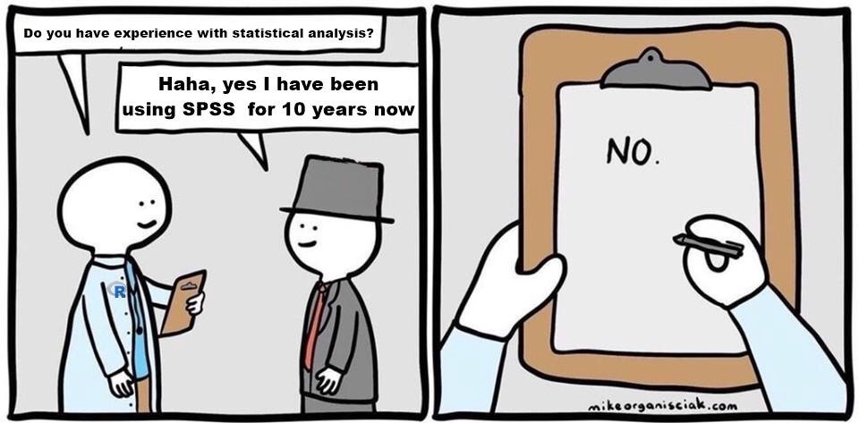
Why R?

• Many alternatives:
  • STATA v.s. R v.s. Python v.s MATLAB v.s. Julia v.s. C/C++
  • No clear answer…
• Advantages of R
  • R is free and open source (v.s. STATA and MATLAB)
  • Designed for data work. Favored by the academia, particular the statistics and econometrics community, which means most of the times you can apply most up-to-date methods with packages developed by the authors. (v.s. all others)
  • R is very flexible and powerful — adaptable to nearly any task, e.g., ’metrics, spatial data analysis, machine learning, web scraping, data cleaning, website building, teaching.
    • Well-developed environment. Rich sources of packages. (v.s. Julia.)
  • R imposes no limitations on your amount of observations, variables, memory, or processing power. (v.s. Stata)
  • If you put in the work, you will come away with a valuable and marketable tool.

Python?

Yes!

• … but … path dependencies of econoemtricians and statisticians
• You got to master one of them first
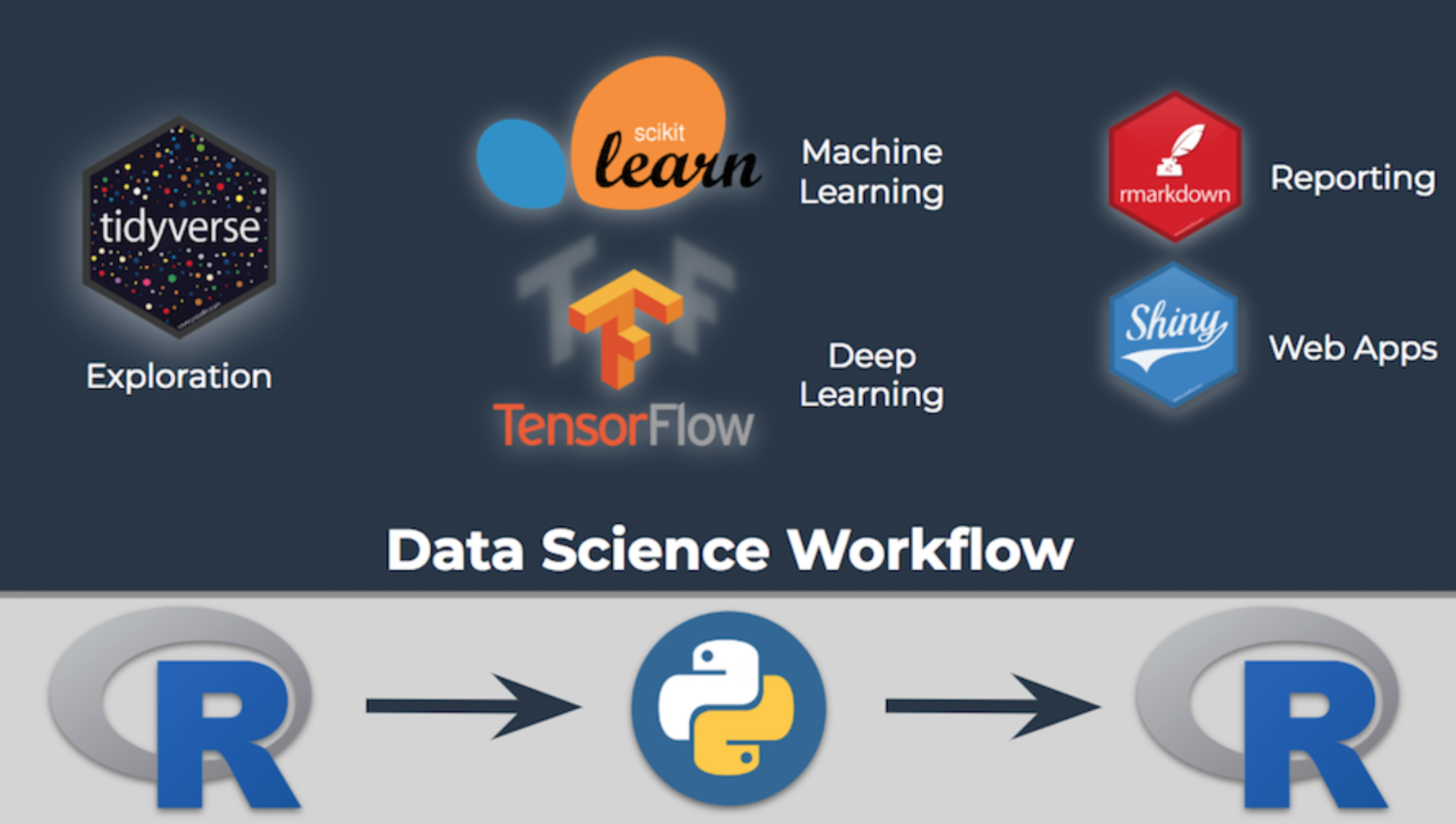
      … and you will be using both of them in the real world

Why R? (cont.)

and you have to learn one of them

Additional resources

• Official Manual
  • R-Introduction
• Books
  • Grolemund G. Hands-On Programming with R
  • Hanck, C., Arnold, M., Gerber, A., and Schmelzer, M. Econometrics with R
• SMU Office of Information Technology Help Desk
• Jenny Bryan’s Happy Git and Github for the useR

Next lecture(s): R programming

---